\(n\)-link Pendulum Benchmark Comparison#
In this notebook we benchmark the n-link pendulum example. This notebook is similar to the \(n\)-link pendulum but is designed for benchmarking kdFlex’s simulation performance and demonstrating how kdlfex’s multibody simulation performance scales.
Requirements:
In this tutorial we will:
Define a method to create the multibody
Run the simulation with increasing number of links
Benchmark simulation runtimes
For a more in-depth descriptions of kdflex concepts see usage.
import os
import gc
import numpy as np
import time
from typing import cast
import pandas as pd
import plotly.express as px
from Karana.Math import IntegratorType
from Karana.Core import discard, allFinalized
from Karana.Frame import FrameContainer
from Karana.Dynamics import (
    Multibody,
    PhysicalBody,
    PhysicalBody,
    HingeType,
    StatePropagator,
    TimedEvent,
    PhysicalBodyParams,
)
from Karana.Math import SpatialInertia, HomTran
from Karana.Models import UniformGravity
Define a Method to Create the Multibody#
Define a method that procedurally creates a n-link multibody for use when we run simulations with increasing number of links. This is the same as in the n-link Pendulum
See Multibody or Frames for more information relating to this step.
def createMbody(fc: FrameContainer, n_links: int):
    """Create the multibody.

    Parameters
    ----------
    n_links : int
        The number of pendulum links to use.
    """
    mb = Multibody("mb", fc)

    # Here, we use the addSerialChain method to add multiple instances of the same body
    # connected in a chain. We add n instances of the pendulum link with the following parameters:
    params = PhysicalBodyParams(
        SpatialInertia(2.0, np.zeros(3), np.diag([3, 2, 1])),
        [np.array([0.0, 1.0, 0.0])],
        HomTran(np.array([0, 0, 0.5])),
        HomTran(np.array([0, 0, -0.5])),
    )
    PhysicalBody.addSerialChain(
        "link", n_links, cast(PhysicalBody, mb.virtualRoot()), htype=HingeType.PIN, params=params
    )

    # finalize and verify the multibody
    mb.ensureCurrent()
    mb.resetData()
    assert allFinalized()

    return mb
Because we run multiple simulations, we write a method ahead of time to cleanup everything whenever the simulation ends. This requires us to delete local variables and discard our containers and scene.
def cleanup():
    """Cleanup the simulation."""
    global integrator, bd1
    del integrator, bd1
    discard(sp)

    gc.collect()

    discard(mb)
    discard(fc)
Run the Simulation With Increasing Number of Links#
Below is the run loop for each simulation. It loops through each sim with an increasing number of links and collects the time it takes to complete.
# Number of links we will run at
n_links_list = [3, 4, 5, 7, 8, 10, 13, 16, 20, 25, 30, 40, 50, 70, 95]

runtimes = []
deriv_calls = []

for n_links in n_links_list:

    # initialization
    fc = FrameContainer("root")
    mb = createMbody(fc, n_links)

    # Set up state propagator and select integrator type: rk4 or cvode
    sp = StatePropagator(mb, integrator_type=IntegratorType.RK4)
    integrator = sp.getIntegrator()

    # add a gravitational model to the state propagator
    ug = UniformGravity("grav_model", sp, mb)
    ug.params.g = np.array([0, 0, -9.81])
    del ug

    # Modify the initial multibody state. Here we will set the first pendulum to 0.5 radians.
    bd1 = mb.getBody("link_0")
    bd1.parentHinge().subhinge(0).setQ([0.5])
    bd1.parentHinge().subhinge(0).setU([0.0])

    # Initialize integrator state
    t_init = np.timedelta64(0, "ns")
    x_init = sp.assembleState()
    sp.setTime(t_init)
    sp.setState(x_init)

    # register the timed event
    h = np.timedelta64(int(1e7), "ns")
    t = TimedEvent("hop_size", h, lambda _: None, False)
    t.period = h
    sp.registerTimedEvent(t)
    del t

    print(f"Number of links: {n_links}")
    start_time = time.time()
    sp.advanceTo(2.0)
    end_time = time.time()
    run_time = end_time - start_time
    runtimes.append(run_time)
    derivs = sp.counters().derivs
    deriv_calls.append(derivs)
    print(f"Time to run: {run_time}, derivs={derivs}")

    # Cleanup
    cleanup()
Number of links: 3
Time to run: 0.5820097923278809, derivs=800
Number of links: 4
Time to run: 0.767350435256958, derivs=800
Number of links: 5
Time to run: 0.9495491981506348, derivs=800
Number of links: 7
Time to run: 1.3216428756713867, derivs=800
Number of links: 8
Time to run: 1.4909248352050781, derivs=800
Number of links: 10
Time to run: 1.8812601566314697, derivs=800
Number of links: 13
Time to run: 2.3990769386291504, derivs=800
Number of links: 16
Time to run: 2.9390172958374023, derivs=800
Number of links: 20
Time to run: 3.665678024291992, derivs=800
Number of links: 25
Time to run: 4.613913536071777, derivs=800
Number of links: 30
Time to run: 5.421594858169556, derivs=800
Number of links: 40
Time to run: 7.2158098220825195, derivs=800
Number of links: 50
Time to run: 8.916121006011963, derivs=800
Number of links: 70
Time to run: 12.402257442474365, derivs=800
Number of links: 95
Benchmark Simulation Runtimes#
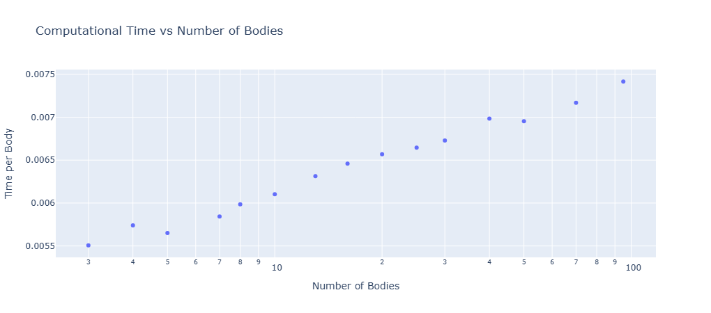
Below the benchmark results are plotted for normalized simulation run times with respect to the number of links. This is the time the simulation takes to run divided by the number of bodies. The Fully Augmented model is compared to the normal simulation style.
normalized_times = np.array(runtimes) / np.array(n_links_list)

run_data_df = pd.DataFrame(
    {
        "NLinks": n_links_list,
        "RunTimes": runtimes,
        "NormalizedTimes": normalized_times,
    }
)

# Create scatter plot
fig = px.scatter(
    run_data_df,
    x="NLinks",
    y="NormalizedTimes",
    title="Computational Time vs Number of Bodies",
    labels={"NLinks": "Number of Bodies", "NormalizedTimes": "Time per Body"},
    log_x=True,
)

# Show plot if not running in a test environment
if not os.getenv("DTEST_RUNNING", False):
    fig.show()
Summary#
Awesome! By running multiple simulations with a varying number of links, you can see that the runtime scales linearly with the number of links.
Further Readings#
Benchmark the n-link pendulum against conventional methods
Simulate collisions with a n-link pendulum