Design notes (Internal)

This area contains assortment of detailed design notes on various topics for the internal development team.

Constraint Embedding

Aggregation Subtree Decomposition

Overview

Many multibody systems have an underlying rooted-tree topology together with constraints that refer to multiple tree nodes. In this document, each such constraint is called a cutjoint. A cutjoint is represented by an unordered list of node IDs rather than by one additional graph edge.

The Aggregation Subtree Decomposition (ASD) identifies tree regions that can be treated as compound or supernodes. The concrete Karana::Core::BasicTreeImpl::aggregationTreeASD() helper performs the tree-related part of this decomposition for one target cutjoint. It does not construct the complete quotient graph.

The central construction is:

1. Find the minimal spanning tree of a cutjoint’s nodes.

2. Treat that spanning tree’s root as the cutjoint’s lowest common ancestor (LCA).

3. Exclude the LCA from the candidate supernode, even when the LCA was explicitly listed in the cutjoint.

4. Resolve proper partial overlaps with candidates from the complete cutjoint list.

5. Return an ordinary directed tree whose root is the final LCA and whose remaining nodes define the supernode.

Scope

This document describes the behavior of:

// Find the ASD subtree associated with one target cutjoint.
std::unique_ptr<Tree<V>> aggregationTreeASD(
    const std::vector<V>& target_cutjoint,
    const std::vector<std::vector<V>>& cutjoints) const;

The method belongs only to the concrete BasicTreeImpl class. It is not part of the abstract Tree interface.

The method returns one target-associated aggregation tree. A higher-level ASD procedure may call this operation while constructing all supernodes and their nesting relationships.

Inputs

Original tree

Let

\[ T = (V, E_T) \]

be a rooted directed tree. Tree edges point from parent to child.

Cutjoint

A cutjoint is a finite node set

\[ C_i \subseteq V \]

containing at least two distinct nodes. The C++ API represents this set as a std::vector<V>.

The vector representation has set semantics:

• Node order is irrelevant.

• Repeated node IDs are ignored.

• Every referenced node must belong to the original tree.

• At least two distinct nodes must remain after duplicates are removed.

For example, {5, 7, 10}, {10, 5, 7}, and {5, 7, 10, 5} represent the same cutjoint.

The second method argument contains the complete cutjoint collection

\[ \mathcal{C} = \{C_1, C_2, \ldots, C_n\}. \]

The target cutjoint must belong to this collection under node-set equality.

Candidate Construction

For a cutjoint \(C_i\), let

\[ H_i = \operatorname{span}_T(C_i) \]

be the minimal subtree of \(T\) that contains every node in \(C_i\). The root of this spanning tree is the common LCA of the cutjoint nodes:

\[ a_i = \operatorname{root}(H_i) = \operatorname{LCA}_T(C_i). \]

The candidate supernode is

\[ S_i = V(H_i) \setminus \{a_i\}. \]

This rule is unconditional: \(a_i\) is excluded even if \(a_i \in C_i\). Consequently, the explicitly listed cutjoint nodes are not required to be a subset of the candidate supernode.

The precise spanning-tree requirement is therefore:

\[ S_i = V(H_i) \setminus \{a_i\}. \]

The figures below use red for an excluded LCA, blue for an explicitly listed node that belongs to the candidate, and green for an included connector node. Dashed green boundaries identify complete candidate supernodes.

Figure 1: Multi-node cutjoint

Consider the cutjoint \(C = \{5, 10, 11\}\). Nodes labeled listed were explicitly listed in the cutjoint.

Node 7 is included because it connects listed node 10 to the spanning-tree root. Node 3 is excluded because it is the LCA and becomes the returned-tree root.

Figure 2: A listed cutjoint node is the LCA

Now consider \(C = \{3, 10\}\), where 3 is an ancestor of 10.

Although node 3 was explicitly listed, it is still excluded. This is not an exception or an error: cutjoint membership identifies the spanning tree, while the LCA-exclusion rule defines the candidate supernode.

The same rule applies when the LCA is the original tree root. The original root is allowed as the returned aggregation-tree root and remains outside the supernode.

Candidate Representation

Conceptually, each candidate stores two pieces of information:

\[ K_i = (S_i, a_i), \]

where:

• \(S_i\) is the LCA-excluded candidate node set.

• \(a_i\) is the excluded candidate LCA.

Keeping the LCA as metadata is necessary because absorbed candidates may have different LCAs. Their LCAs determine the root of the final returned tree.

Selecting the Target Candidate

The first argument identifies one target cutjoint \(C_t\). Before candidate construction, the method:

1. Normalizes every cutjoint by removing repeated nodes.

2. Validates all referenced nodes.

3. Verifies that every normalized cutjoint contains at least two nodes.

4. Finds a set-equal copy of \(C_t\) in the complete collection \(\mathcal{C}\).

If the target does not occur in the complete collection, the method rejects the request.

The initial aggregation region is the target candidate:

\[ S \leftarrow S_t. \]

Its initial LCA collection is

\[ A \leftarrow \{a_t\}. \]

Overlap Resolution

Proper partial overlap

A pool candidate \(S_i\) merges with the current region \(S\) only when the two sets overlap and neither contains the other:

\[ S \cap S_i \neq \varnothing, \]

\[ S \nsubseteq S_i, \]

and

\[ S_i \nsubseteq S. \]

This relationship is called proper partial overlap.

When it occurs, the method updates

\[ S \leftarrow S \cup S_i \]

and records \(a_i\) in the component LCA collection \(A\).

Containment represents nesting

Containment alone does not cause a merge. If

\[ S_i \subseteq S \]

or

\[ S \subseteq S_i, \]

the candidates can represent nested supernodes and remain separate.

Equal candidates also require no merge.

Shared LCAs do not imply overlap

Candidate LCAs are excluded before overlap testing. Two candidates that share only an LCA therefore remain separate.

For example, cutjoints {3, 10} and {3, 5} have the same LCA 3, but their candidates {7, 10} and {5} are disjoint.

Figure 3: Partial overlap versus containment

Proper partial overlap merges candidate \(A = \{10, 12\}\) and candidate \(B = \{10, 14\}\) at node 10:

Containment remains nested:

Selecting the inner candidate returns supernode {10}. Selecting the outer candidate returns supernode {5, 7, 10}. Containment alone does not combine them.

Transitive closure

Overlap resolution runs to a fixed point. A merge may add nodes that create a proper partial overlap with a candidate examined earlier. The method therefore rescans the candidate pool until a complete pass makes no change.

Final LCA

Suppose the target candidate and all candidates absorbed by proper partial overlap have LCA metadata

\[ A = \{a_{i_1}, a_{i_2}, \ldots, a_{i_k}\}. \]

The final returned-tree root is

\[ a = \operatorname{LCA}_T(A). \]

A merge may therefore move the returned LCA upward. The LCA is not fixed to the target candidate’s original LCA.

The final LCA may be the original tree root. This is valid and does not require special rejection.

An individual candidate LCA is excluded from that candidate. After merging, it may nevertheless occur inside the final supernode if another candidate’s spanning tree contains it. Only the final returned-tree root \(a\) is guaranteed to be external to the returned supernode.

Returned Tree

The method returns an ordinary directed tree containing:

\[ V_R = \{a\} \cup S, \]

where \(a\) is the final LCA and \(S\) is the merged supernode node set.

The interpretation is:

returned_tree.root()              final LCA; not in the supernode
all other returned-tree vertices  nodes in the supernode

Original tree edges are reused to connect the returned vertices. Every supernode vertex must have its original parent either inside the supernode or equal to the returned root. Otherwise, the selected union cannot be represented as one valid returned subtree and the method rejects it.

Figure 4: Returned-tree interpretation

Only the nodes inside the dashed boundary define the supernode. The returned root a is present in the ordinary tree but excluded from the supernode.

Cutjoint relationships are not inserted as edges in the returned tree. The result stores only original directed-tree topology.

Algorithm

function aggregationTreeASD(target_cutjoint, cutjoints):
    normalized_pool = []

    for cutjoint in cutjoints:
        nodes = validate_and_remove_duplicates(cutjoint)
        normalized_pool.append(nodes)

    target = validate_and_remove_duplicates(target_cutjoint)

    if no node-set-equal target exists in normalized_pool:
        reject the request

    selected = candidate_from_spanning_tree(target)
    candidates = candidate_from_spanning_tree(c) for c in normalized_pool

    aggregation_nodes = selected.nodes
    component_lcas = [selected.lca]
    absorbed = [false for each candidate]

    changed = true
    while changed:
        changed = false

        for candidate in candidates:
            if candidate was already absorbed:
                continue

            if candidate contains aggregation_nodes:
                continue  // Preserve nesting.

            if aggregation_nodes contains candidate.nodes:
                continue  // Preserve nesting or equality.

            if candidate.nodes intersects aggregation_nodes:
                aggregation_nodes = aggregation_nodes union candidate.nodes
                component_lcas.append(candidate.lca)
                mark candidate absorbed
                changed = true

    final_lca = common_lca(component_lcas)

    return original_tree_subtree(
        root = final_lca,
        remaining_nodes = aggregation_nodes)

Required Behaviors

LCA exclusion

For every independently generated candidate,

\[ a_i \notin S_i. \]

This remains true when \(a_i\) was explicitly listed in \(C_i\).

Spanning-tree coverage

Every non-root node of a cutjoint’s minimal spanning tree belongs to its candidate:

\[ V(H_i) \setminus \{a_i\} = S_i. \]

This replaces the obsolete requirement that every explicitly listed cutjoint node must belong to the candidate.

Original-root acceptance

The original tree root is allowed to be a candidate LCA or the final merged LCA. It is returned as the aggregation-tree root and excluded from the supernode in the usual way.

Target membership

The target cutjoint must occur in the complete cutjoint collection under node-set equality.

Nested containment

Candidate equality or containment does not enlarge the target region. This permits an inner supernode to be represented independently inside a later outer supernode.

Proper-overlap closure

All candidates connected to the selected region through transitive proper partial overlap are absorbed.

Deterministic topology

Input order and duplicate cutjoint nodes do not affect candidate membership or the returned topology. Returned vertices are assembled in the original tree’s topological order.

Invalid Inputs and Ill-posed Results

The method rejects:

• A cutjoint containing fewer than two distinct nodes.

• A cutjoint referring to a node absent from the original tree.

• A target cutjoint absent from the complete cutjoint collection.

• A merged node set that cannot be connected through the final LCA using the original parent edges included in the returned tree.

The method does not reject a result merely because its LCA is the original tree root.

Relationship to Full ASD

aggregationTreeASD() performs the graph-related work needed to identify the candidate associated with one target cutjoint and its proper-overlap component. It does not itself:

• Replace original nodes with compound-body nodes.

• Construct every nested supernode in one call.

• Build the complete quotient tree.

• Transfer physical bodies, joints, or constraints into compound bodies.

Those operations belong to the higher-level decomposition and model-building procedure.

In particular, the phrase cutjoint absorption must not be interpreted as a requirement that every explicitly listed cutjoint node lie inside the supernode. ASD uses the cutjoint node set to locate a spanning tree, then excludes that spanning tree’s LCA by definition.

Summary

For each cutjoint node set \(C_i\):

\[ H_i = \operatorname{span}_T(C_i), \qquad a_i = \operatorname{root}(H_i), \qquad S_i = V(H_i) \setminus \{a_i\}. \]

The target cutjoint must belong to the complete cutjoint collection. Starting from its candidate, the method absorbs candidates connected through transitive proper partial overlap while leaving equal or containing candidates separate for nesting. The common LCA of the absorbed candidates becomes the root of the returned tree. That root is always excluded from the represented supernode, including when it is an explicitly listed cutjoint node or the original tree root.

SDF importers/exporters

Converting kdFlex multibodies to SDF

This leg projects the multibody data in Karana.Dynamics.SOADyn_types.SubGraphDS into an SDF 1.9 model. A Karana.KUtils.BasicPrefab.BasicPrefabDS input is accepted only as a container: the converter selects its params.subtree. Prefab and KModel data are outside the conversion boundary.

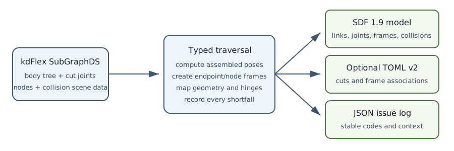
The forward conversion products and their responsibilities.

Process

The converter loads the source through the concrete kdFlex fromFile() API and walks the typed body tree. Each body becomes a link with its mass, center of mass, and inertia tensor. Tree hinges become ordinary SDF joints. Each Karana.Dynamics.SOADyn_types.LoopConstraintCutJointDS becomes an additional joint marked kdflex_loop_joint="true".

kdFlex stores independent parent- and child-body transforms for a connection. SDF ordinarily describes an assembled link pose plus a joint pose. To retain both kdFlex transforms, the exporter creates one frame on each endpoint and chooses the child-link pose so the endpoints coincide:

\[ {}^{P}T_C = {}^{P}T_J ({}^{C}T_J)^{-1}. \]

Sensor, force, and constraint nodes also become body-attached SDF frames at the same translation and orientation. Consequently the reverse leg can recover a node without treating a body origin as a joint location.

Deterministic names

Arbitrary kdFlex names are encoded with URL-safe Base64 without padding. The encoding is reversible and stable, including for spaces or punctuation.

The four forms are:

kdflex__node__ROLES__BODY__NODE
kdflex__joint_parent__JOINT__ROLES__NODE
kdflex__joint_child__JOINT__ROLES__NODE
kdflex__collision__KIND__BODY__NAME__LAYERS__CONVEX

Node names encode roles, body, and node. Endpoint names encode the joint and endpoint node. Collision names encode source kind, body, object name, hexadecimal layer mask, and convexity.

ROLES is a sorted compact token: c means constraint, f force, s sensor, and n no node role. KIND is part or file.

The exporter also writes MODEL.sdf.kdflex.toml. Its cut_joints, joint_endpoints, and node_frames entries allow the reverse leg to interpret an SDF whose deterministic names have been edited. The generated SDF remains self-describing without this optional file.

Collision geometry

Only kdFlex scene objects whose layer mask contains Karana.Scene.LAYER_COLLISION become SDF collision elements. The exact supported subset is:

kdFlex source	SDF target	Important restriction
BoxGeometry	box	dimensions include the three-axis scale
SphereGeometry	sphere	scale must be uniform
CylinderGeometry	cylinder	the two radial scales must match
CapsuleGeometry	capsule	the two radial scales must match
StaticMeshGeometry	mesh	a filename is required
SceneFileObjectSpec	mesh	its scalar scale is repeated on three axes

Object pose is copied. The deterministic name carries the original layer mask, object name, source kind, and mesh is_convex flag because SDF collision geometry has no equivalent kdFlex metadata fields. Material and contact behavior are not transferred.

Issue log

Every invocation creates JSON at OUTPUT.errors.log, including successful conversions with an empty entries array. --error-log PATH selects another location. Each entry has severity, a stable code, a human-readable message, and object-specific context. Unsupported hinges are exported as fixed and logged. Unsupported constraints and inexact collision shapes are logged; collision shapes that cannot be represented exactly are skipped.

Review this file before accepting a conversion. A zero process exit status means the conversion completed, not necessarily that the issue count is zero.

Gaps and caveats

• Unsupported kdFlex hinge families become fixed SDF joints and are logged.

• Only position bounds are transferred; joint dynamics, coupling, prescribed state, and coordinate constraints are not.

• General constraint frames, inb_nodal_matrix, and virtual-root scene data are not represented.

• Collision contact, friction, filtering, material, and self-collision settings are not transferred.

• Visual mesh URIs are copied as written and may not remain portable.

• SI values replace the source unit spelling and numeric formatting.

• Base-body attachment to the kdFlex virtual root is implicit in SDF.

See the detailed forward gap register and the reverse guide.

Command

python3 kdflex_sdf_datastruct_converter.py to-sdf \
  input.yaml model.sdf --error-log model.forward.errors.log

Converting SDF graphs to kdFlex multibodies

This leg converts one direct SDF model into Karana.Dynamics.SOADyn_types.SubGraphDS. The complete link-and-joint graph is considered; the input is not required to be a tree.

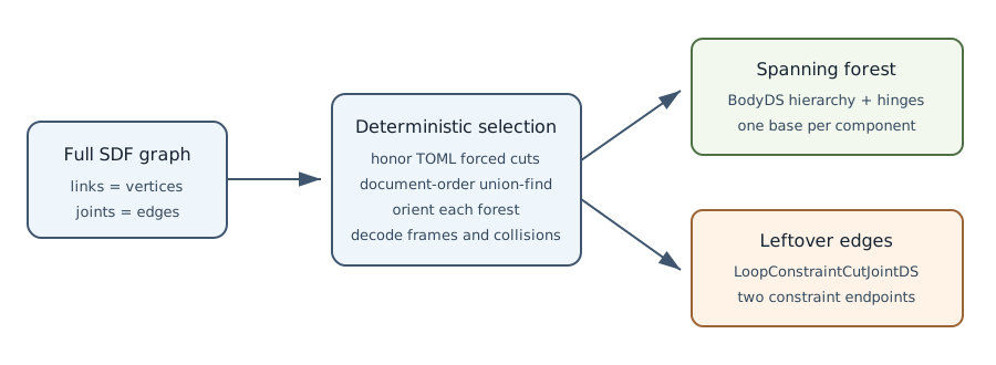
Graph decomposition and DataStruct construction in the reverse leg.

Process

Links are graph vertices and joints are undirected edges during selection. The converter first honors any joints listed in the optional TOML cut_joints array. It then applies deterministic document-order union-find to the remaining edges. Accepted edges form a spanning forest; cycle-producing and policy-cut edges are leftovers.

Each forest is oriented into the single-parent hierarchy required by kdFlex. Its root becomes a base body with a FULL6DOF virtual-root hinge. Tree edges become body hinges, while every leftover edge becomes a Karana.Dynamics.SOADyn_types.LoopConstraintCutJointDS. Edge reversal during orientation also swaps endpoint roles, preserving local transforms.

The converter constructs a real SubGraphDS, saves it with toFile(), reloads it, and validates the concrete type. It does not parse or synthesize kdFlex YAML dictionaries.

Naming and optional TOML

Files written by the forward converter carry reversible kdflex__node__..., kdflex__joint_parent__..., kdflex__joint_child__..., and kdflex__collision__... names. The reverse leg decodes these names directly, so a sidecar is not essential.

If MODEL.sdf.kdflex.toml exists, it is loaded automatically. Use --edge-sidecar FILE to override that location. Version 2 uses this structure:

format_version = 2
cut_joints = ["steering_loop"]

[[joint_endpoints]]
joint = "steering_loop"
parent_frame = "parent_marker"
child_frame = "child_marker"

[[node_frames]]
frame = "camera_marker"
body = "chassis"
name = "camera_mount"
roles = ["sensor"]

This is particularly useful for externally authored or renamed SDF. It cannot create pose information that is absent or resolve arbitrary semantic frame chains.

Collision geometry

Direct link collisions containing box, sphere, cylinder, or capsule geometry become collision-layer ScenePartSpec objects. A uniformly scaled mesh becomes a SceneFileObjectSpec. Converter-generated names restore the original kdFlex name, layers, source kind, and mesh convexity; ordinary SDF collisions receive collision-only defaults.

Plane, heightmap, ellipsoid, polyline, and other unsupported shapes are skipped and logged. A mesh with unequal scale components is skipped because the target DataStruct has only scalar scale. Collision surface data is not represented by these scene DataStructs and generates an omission entry.

Issue log

Every invocation creates OUTPUT.errors.log; --error-log PATH overrides it. Entries have stable codes and context for the affected joint, constraint, frame, body, or collision. Fatal exceptions are also recorded as CONVERSION_FAILED before being re-raised. Treat the log as part of the conversion result and archive it with the SDF, optional TOML, and kdFlex file.

Gaps and caveats

• Only fixed, revolute/continuous, prismatic, universal/revolute2, and ball joints have mappings. Unsupported types fail conversion and are logged.

• Arbitrary SDF pose-frame graphs, nested models, worlds, includes, and joints to world are not resolved.

• Without endpoint frames, a conventional SDF joint provides only one local attachment pose; the other kdFlex endpoint uses identity.

• Tree choice can alter hierarchy and coordinate signs. TOML can force cuts but cannot force a root or force an edge into the tree.

• Axis expressed_in, dynamics, most limits, mimic/gearbox behavior, plugins, and initial state are omitted.

• A rotated SDF inertial frame is not applied to the imported inertia tensor.

• Visuals and SDF sensor elements do not become kdFlex scene objects or nodes.

• General constraint frames, virtual-root scene data, and inb_nodal_matrix are not constructed.

The regression checks all supported body and node poses and compares the full 6×6 overall multibody spatial-inertia matrix through the kdFlex runtime API. Those checks establish preservation for the covered model; they do not make an unsupported logged feature lossless.

See the detailed reverse gap register and the forward guide.

Command

python3 kdflex_sdf_datastruct_converter.py to-kdflex \
  model.sdf output.json --edge-sidecar model.sdf.kdflex.toml \
  --error-log output.reverse.errors.log

Using Atmosphere and Aerodynamics Models Together

Written by Codex for jain on 2026-08-06.

Overall goal

An atmospheric-flight simulation must answer two different questions at every integration step:

1. What air surrounds the vehicle here and now? The atmosphere model supplies density, wind, and other environmental properties.

2. What loads does that air create on this vehicle? The aerodynamics model combines the atmospheric state with vehicle motion, geometry, and aerodynamic coefficients to produce force and moment.

Keeping these responsibilities separate lets the same vehicle aerodynamics run on Earth, Mars, or another atmospheric body. It also lets a developer replace a simple standard atmosphere with a high-fidelity model without rewriting the vehicle equations.

        flowchart LR
    S[Simulation time and vehicle state]
    F[Planet-fixed atmosphere frame]
    P[AtmosphereProvider adapter]
    C[Atmosphere modeling core]
    A[AerodynamicsDamped KModel]
    L[Force and moment on vehicle nodes]

    S --> A
    F --> A
    A -->|time and Cartesian position| P
    P -->|planet-specific coordinates| C
    C -->|density, wind, temperature,<br/>pressure, speed of sound| P
    P -->|AtmosphereState| A
    A --> L
    

The important boundary is the provider adapter. The aerodynamic model knows which frame contains the atmosphere, but it does not know the planet’s radius, ellipsoid, geodetic convention, rotation rate, or atmosphere product.

The aerodynamics model

The C++ Karana::Models::AerodynamicsDamped KModel is implemented in the neighboring header. Its standalone AerodynamicsDampedCore computes quasi-steady lift, drag, side force, static moments, and angular-rate damping. The thin KModel wrapper obtains live kdFlex frame kinematics and applies a Karana::Math::SpatialForce to each configured force node.

For each aerodynamic surface, the simulation provides:

• A kdFlex force node whose local axes are +X forward, +Y right, and +Z down.

• Reference area, chord, span, and aerodynamic coefficients.

• A planet- or atmosphere-fixed frame.

• Either a unified atmosphere provider or simpler density and wind callbacks.

The KModel determines the surface velocity relative to the atmosphere frame. Consequently, a rotating body-fixed frame automatically accounts for the planet’s rotation. The simulation must not add the surface velocity caused by planetary rotation a second time.

The principal load relationship is

\[ \bar q = \frac{1}{2}\rho\lVert\mathbf V_{air}\rVert^2, \]

where \(\rho\) comes from the atmosphere provider and \(\mathbf V_{air}\) is the surface velocity relative to the air. The model multiplies dynamic pressure by the configured reference geometry and coefficients to obtain force and moment.

See README.md for all coefficient equations, axis conventions, physics references, build instructions, and tests.

The general-purpose atmosphere provider

AerodynamicsDamped::AtmosphereProvider is the preferred integration point for a coupled atmosphere model. It has the conceptual C++ signature:

AtmosphereState provider(double time_s, const km::Vec3 &position_m);

The arguments have deliberately planet-neutral meanings:

• time_s is elapsed simulation time in seconds.

• position_m is the surface position in the axes of the atmosphere frame supplied when the KModel was created.

The returned AtmosphereState contains:

Field	Meaning	Units used by the C++ interface
density_kg_m3	Atmospheric mass density	kg/m³
wind_velocity_in_atmosphere	Wind resolved in atmosphere-frame axes	m/s
temperature_k	Temperature, when available	K
pressure_pa	Static pressure, when available	Pa
speed_of_sound_m_s	Local speed of sound, when available	m/s

Aerodynamics currently consumes density and wind. Temperature, pressure, and speed of sound are carried for diagnostics and future compressibility models. Unavailable optional scalar fields default to NaN.

The provider is called once per surface during each derivative evaluation. It therefore produces one internally consistent sample rather than asking a stateful atmosphere separately for density and wind.

Simpler density and wind providers

For an analytic or constant environment, separate callbacks remain available:

density_provider(time_s, position_m) -> density_kg_m3
wind_provider(time_s, position_m) -> wind_velocity_in_atmosphere_m_s

Do not supply these callbacks together with AtmosphereProvider; the KModel rejects that ambiguous configuration. With no density callback, the model uses params.air_density_kg_m3. With no wind callback, the air is stationary in the configured atmosphere frame.

        sequenceDiagram
    participant I as kdFlex integrator
    participant K as AerodynamicsDamped
    participant P as AtmosphereProvider
    participant C as Planet atmosphere core
    participant N as Vehicle force node

    I->>K: preDeriv(time, state)
    K->>K: Read surface pose and relative velocity
    K->>P: sample(time_s, position in atmosphere frame)
    P->>C: Convert coordinates and evaluate model
    C-->>P: Native atmospheric state
    P-->>K: AtmosphereState
    K->>K: Compute dynamic pressure and aerodynamic loads
    K->>N: Accumulate SpatialForce
    

The atmospheric modeling core

An atmospheric core contains the actual environmental physics or empirical data model. It should be usable without constructing a kdFlex multibody or KModel. Typical inputs include:

• A model epoch and elapsed time.

• Planet-specific longitude, latitude, and altitude.

• Solar and geomagnetic activity, season, or weather data.

• Model configuration and data-file locations.

Typical outputs are density, temperature, pressure, speed of sound, and local wind. A core may use geodetic coordinates, planetocentric coordinates, areoid height, or another native convention. Those details belong behind the adapter.

This separation is useful for testing. The atmosphere core can be checked against its publisher’s reference cases, while the provider can be tested for coordinate order, frame direction, units, and wind-vector transformation.

Adapting the Earth atmosphere

The standalone Karana::EarthGram::Atmosphere core in /workspace/code/EarthGRAM wraps NASA Earth-GRAM. It accepts geodetic longitude, latitude, altitude, and elapsed time. It does not know the vehicle’s kdFlex frames.

An Earth adapter therefore performs these steps:

1. Receive elapsed time and Cartesian position in an Earth-fixed frame such as ITRF93.

2. Use TerrainGrid.createEarthWGS84() and TerrainGrid.fromCartesianVertex() to obtain longitude, latitude, and altitude, in that order.

3. Populate an Earth-GRAM GeodeticPoint and sample the standalone core.

4. Copy density, temperature, pressure, and speed of sound into AtmosphereState.

5. If wind is enabled, transform Earth-GRAM’s local east-north-up wind into the Cartesian axes of the Earth-fixed atmosphere frame before returning it.

        flowchart TD
    E[ITRF93 Cartesian position]
    W[WGS-84 TerrainGrid]
    G[Longitude, latitude, altitude]
    EG[Earth-GRAM core]
    ENU[Earth-GRAM local ENU wind]
    EC[Earth-fixed Cartesian wind]
    AS[AtmosphereState]

    E --> W --> G --> EG
    EG --> AS
    EG --> ENU -->|local-to-Earth-fixed transform| EC --> AS
    

The NESC orbital implementation provides a working density-and-temperature example in orbital_case.py. Its Earth-specific WGS-84 conversion is intentionally outside AerodynamicsDamped.

Earth-GRAM runtime and deployment dependencies

An atmosphere adapter can be correct in code and still fail at startup if its data products or kernels are not deployed. Treat these files as part of the simulation configuration, record their versions, and check them before a long run.

Earth-GRAM’s Config.data_root names the directory that contains the modeldata and NCEPdata subdirectories. The workspace default is:

/workspace/DATA/GramSuite/Earth/data

With that default, the current NCEP/MET configuration expects this layout:

/workspace/DATA/GramSuite/Earth/data/
├── modeldata/
│   ├── sdata.txt
│   ├── topo.txt
│   └── zdata.txt
└── NCEPdata/
    └── FixedBin/
        ├── Nb971501.bin
        ├── ...
        └── Nb971512.bin

The three modeldata files are runtime dependencies, not examples:

File	Earth-GRAM purpose
sdata.txt	Stationary perturbation data
topo.txt	Topographical data
zdata.txt	Zonal-mean data

The twelve Nb9715MM.bin files cover the calendar months for the configured 1997–2015 NCEP climatology. A run opens the binary matching its configured month. Keeping all twelve allows the same installation to run any month.

Config.spice_root separately names a directory with three required subdirectories. The workspace default is /workspace/code/EarthGRAM/resources/spice and resolves to:

spice_root/
├── lsk/naif0012.tls
├── pck/pck00011.tpc
└── spice/de442s.bsp

The current files may be symbolic links, but every link target must remain readable in the runtime environment. The leap-second kernel establishes time conversion, the text PCK supplies planetary constants, and the BSP supplies the Earth/Sun ephemeris used by Earth-GRAM.

Dependency	Build time	Runtime	Notes
GramSuite headers	Yes	No	Compile the standalone wrapper
Earth/GRAMCommon static libraries	Yes	No	Linked into the wrapper
CSPICE headers and static library	Yes	No	Linked into the wrapper
modeldata files	No	Yes	All three files are required
NCEP FixedBin data	No	Yes	At least the run’s month is required
Earth-GRAM SPICE kernels	No	Yes	LSK, PCK, and BSP are required
Earth texture	No	No	Visualization only

The GramSuite sample_inputs directory is not a runtime dependency. It is useful only for vendor examples and independent regression comparisons.

Relocating the runtime data

The files do not have to remain under /workspace. Set both roots before constructing the stateful Earth-GRAM atmosphere:

config.data_root = "/opt/atmosphere/Earth/data"
config.spice_root = "/opt/atmosphere/Earth/spice"
earth_atmosphere = keg.Atmosphere(config)

Earth-GRAM will then expect modeldata/sdata.txt, modeldata/topo.txt, modeldata/zdata.txt, and NCEPdata/FixedBin beneath the new data_root. It will expect lsk, pck, and spice beneath the new spice_root.

For reproducible deployment, validate the directories, individual files, permissions, symbolic-link targets, and model versions during simulation startup. Checking only that the root directory exists is not sufficient to prove that every later atmosphere query can load its data.

Switching to another planetary atmosphere

Changing planets should require a new frame and provider adapter, not a new aerodynamics model.

For Mars, for example:

1. Supply a Mars body-fixed atmosphere frame to AerodynamicsDamped.

2. Implement a Mars adapter with the same (time_s, position_m) contract.

3. Convert Mars-fixed Cartesian position using the ellipsoid, areoid, or planetocentric convention required by the selected Mars atmosphere core.

4. Configure and call Mars-GRAM or another Mars atmosphere implementation.

5. Transform any local north-east-down or east-north-up wind into Mars-fixed Cartesian axes.

6. Return the common AtmosphereState.

No WGS-84, ITRF93, Earth rotation rate, or Earth-GRAM type should appear in the Mars adapter. Conversely, no Mars datum or Mars-GRAM type should enter AerodynamicsDamped.

Concern	Earth implementation	Mars implementation	Shared component
Atmosphere frame	ITRF93	Mars-fixed	Frame passed to KModel
Coordinates	WGS-84	Mars datum	Provider adapter pattern
Atmosphere physics	Earth-GRAM	Mars-GRAM or equivalent	AtmosphereState
Vehicle coefficients	Unchanged	Unchanged	AerodynamicsDamped
Load application	Unchanged	Unchanged	kdFlex force nodes

Basic integration example

The following Python excerpt assumes that the simulation has already created a state propagator, a vehicle force node, and an Earth-fixed frame. It shows the important provider boundary without obscuring it with complete vehicle setup.

import numpy as np

import Karana.Math as km
from Karana.Math.Kquantities import ureg
from Karana.Scene._Terrain_Py import TerrainGrid

import _AerodynamicsDamped_Py as kad
import _EarthGRAM_Py as keg


terrain = TerrainGrid.createEarthWGS84()
earth_atmosphere = keg.Atmosphere(earth_gram_config)


def atmosphereProvider(time_s: float, position_m: np.ndarray) -> kad.AtmosphereState:
    """Convert an Earth-fixed point and return one coherent atmosphere sample."""
    # TerrainGrid returns longitude first, followed by latitude and altitude.
    longitude, latitude, altitude = terrain.fromCartesianVertex(position_m)

    point = keg.GeodeticPoint()
    point.elapsed_time = time_s
    point.longitude = float(longitude)
    point.latitude = float(latitude)
    point.altitude = float(altitude)
    earth_state = earth_atmosphere.sample(point)

    state = kad.AtmosphereState()
    state.density_kg_m3 = earth_state.density
    state.temperature_k = earth_state.temperature
    state.pressure_pa = earth_state.pressure
    state.speed_of_sound_m_s = earth_state.speed_of_sound

    # This minimal example chooses still air in the rotating Earth-fixed frame.
    # A wind-enabled adapter must transform Earth-GRAM ENU wind to Earth-fixed
    # Cartesian axes before assigning this field.
    state.wind_velocity_in_atmosphere = np.zeros(3) * ureg.meter / ureg.second
    return state


aerodynamics = kad.AerodynamicsDamped.create(
    "vehicle_aerodynamics",
    propagator,
    [aerodynamic_force_node],
    earth_fixed_frame,
    None,  # No separate density provider.
    None,  # No separate wind provider.
    None,  # Use the built-in coefficient model, not a custom load provider.
    atmosphereProvider,
)

surface = kad.AeroSurfaceConfig()
surface.name = "vehicle_reference_surface"
surface.area_m2 = 12.0
surface.chord_m = 2.0
surface.span_m = 8.0
surface.cl0 = 0.2
surface.cl_alpha = 4.5
surface.cd0 = 0.03
surface.induced_drag_factor = 0.05
aerodynamics.params.surfaces = [surface]

# Ask kdFlex to validate the completed model graph after configuration.
propagator.ensureHealthy()

The C++ KModel automatically converts compatible Python quantities at its quantity-aware properties. The plain numeric fields in AtmosphereState use the SI units listed earlier.

Summary recipe

Use this checklist when adding atmospheric aerodynamics to a vehicle:

1. Build vehicle dynamics. Create the multibody, propagator, physical body, and one force node for each aerodynamic surface.

2. Choose the atmosphere frame. Use the rotating body-fixed frame expected by the environmental model.

3. Configure the atmosphere core. Set its epoch, environmental indices, data paths, and planet-specific options. Verify every required runtime data file and kernel before constructing the atmosphere.

4. Write a thin provider adapter. Convert body-fixed Cartesian position to the core’s native coordinates, evaluate it once, transform wind into atmosphere-frame Cartesian axes, and return AtmosphereState.

5. Create AerodynamicsDamped. Pass the propagator, surface nodes, atmosphere frame, and unified provider.

6. Configure surfaces. Supply geometry and coefficients in each node’s local aerodynamic axes.

7. Validate conventions. Test coordinate order, altitude datum, wind sign, frame axes, units, and a zero-wind case before running a full trajectory.

8. Validate lifecycle and physics. Run a short simulation and cleanup test, then compare the atmosphere and trajectory with independent reference data.

Following this recipe keeps vehicle aerodynamics reusable while placing every planet-specific decision in a small, testable atmosphere adapter.

NESC Flight Dynamics Check Cases

NESC 2015 kdFlex Check-Case Overview

Written by Codex for jain on 2026-08-06.

Purpose and scope

This workspace ports the NASA Engineering and Safety Center (NESC) 2015 six-degree-of-freedom flight-simulation check cases to kdFlex. The cases are verification problems, not one “correct” reference trajectory. NASA collected independent submissions from several simulation tools so that developers could compare equations of motion, frames, environment models, vehicle models, and integration behavior.

The workspace contains two related suites:

• atmospheric: falling bodies, cannonballs, controlled F-16 maneuvers, and a two-stage launch vehicle.

• orbital: ISS, sphere, and cylinder cases that progressively add gravity harmonics, third bodies, atmosphere, applied loads, rigid-body rotation, and gravity-gradient torque.

Together they contain 45 implemented case directories: 19 atmospheric scenarios or subcases and 26 orbital scenarios or subcases.

NASA did not complete Atmospheric Case 14 because of resource constraints. The published orbital sequence begins at Case 02. Those numbering gaps are therefore part of the source assessment, not missing folders in this port.

The primary source is the NASA NESC 2015 check-case website, which provides scenario descriptions, DAVE-ML models, initial conditions, raw trajectories, plotting tools, specifications, and errata. The accompanying Volume I report gives the assessment overview, while Volume II contains detailed definitions and comparisons.

        flowchart LR
    N[NASA definitions, models,<br/>errata, and trajectories]
    C[Typed case configuration]
    E[Shared kdFlex engine]
    P[Selected physics branches]
    O[NASA-shaped CSV output]
    V[Comparison with independent<br/>NASA submissions]

    N --> C --> E --> P --> O --> V
    

Atmospheric cases

Simple-body progression

Cases 01 through 10 deliberately add one modeling feature at a time. This makes a discrepancy easier to associate with drag, rotational damping, geodesy, gravity, Earth rotation, or wind.

Case	Scenario	Main verification focus
01	Dragless dropped sphere	WGS-84/J2 free fall
02	Tumbling brick, no damping	6-DOF rotation without aero torque
03	Tumbling brick with damping	Angular-rate aero moments
04	Dropped sphere, round Earth	Stationary sphere and point gravity
05	Dropped sphere, rotating Earth	Air-relative velocity from rotation
06	Dropped sphere, WGS-84	Oblate geodesy and J2 gravity
07	Dropped sphere, steady wind	Constant local-east wind
08	Dropped sphere, wind shear	Altitude-dependent local-east wind
09	Eastward cannonball	Horizontal launch and rotating WGS-84
10	Northward cannonball	Meridian flight and frame conventions

F-16 and launch-vehicle progression

Case	Scenario	Main verification focus
11	Subsonic F-16 trim	Open-loop low-speed trim flyout
12	Supersonic F-16 trim	High-Mach aero and propulsion tables
13.1	F-16 altitude step	Closed-loop longitudinal response
13.2	F-16 airspeed step	Throttle and speed control
13.3	F-16 heading step	Lateral-directional control
13.4	F-16 lateral step	Navigation and lateral position control
15	F-16 near the North Pole	Polar navigation singularity handling
16	F-16 at the date line	Longitude wrapping and guidance continuity
17	Unguided two-stage rocket	Staging, variable mass, thrust, and ascent

Orbital cases

The orbital suite starts with an eight-hour ISS propagation and then isolates or combines environmental and rigid-body effects.

Case	Scenario	Main verification focus
02	ISS, spherical Earth	Kepler propagation and J2000/ITRF93 output
03A	ISS, GEM-T1 4×4	Harmonic coefficient normalization
03B	ISS, GEM-T1 8×8	Higher-degree rotating gravity field
04	ISS with Sun and Moon	Differential third-body gravity
05A	Elliptical ISS, minimum MET	Low solar-activity atmosphere output
05B	Elliptical ISS, mean MET	Mean solar-activity atmosphere output
05C	Elliptical ISS, maximum MET	High solar-activity atmosphere output
06A	Sphere with fixed drag	Constant density and Earth-relative speed
06B	Sphere with dynamic drag	Live MET density coupled to drag
06C	Cylinder plane change	Finite-duration cross-track thrust
06D	Cylinder Earth departure	Finite-duration along-track thrust
07A	Sphere, 4×4 plus third bodies	Combined gravity without drag
07B	Sphere, 8×8 plus third bodies	Higher-degree combined gravity
07C	Case 07A plus drag	4×4 gravity, third bodies, and MET drag
07D	Case 07B plus drag	8×8 gravity, third bodies, and MET drag
08A	ISS free rotation, zero rate	Inertially fixed attitude
08B	ISS free rotation, initial rate	Torque-free asymmetric rigid body
09A	ISS torque, zero rate	Scheduled body torque
09B	ISS torque, initial rate	Torque plus existing rotation
09C	ISS force and torque, zero rate	Coupled translation and rotation
09D	ISS force and torque, initial rate	Coupled loads with body rotation
10A	Circular cylinder, zero offset	Gravity-gradient torque
10B	Circular cylinder, rate offset	Gravity gradient plus rate offset
10C	Elliptical cylinder, zero offset	Time-varying gravity gradient
10D	Elliptical cylinder, rate offset	Elliptical case with rate offset
FULL	Elliptical ISS, all effects	Coupled environment and attitude

General kdFlex modeling approach

The port uses a common architecture instead of reproducing each case as a large independent script. A small launcher selects an immutable, typed case configuration. A shared engine creates the kdFlex object graph and activates the required physics. This keeps a correction to frames, units, or force application consistent across every affected case.

        flowchart TD
    L[Small case launcher]
    T[Frozen typed configuration]
    S[Shared simulation engine]
    R[Reference frames and transforms]
    B[Multibody, rigid body, and force nodes]
    M[Gravity, atmosphere, aero,<br/>propulsion, and applied-load models]
    I[StatePropagator and RK4 integration]
    CSV[Case CSV writer]

    L --> T --> S
    S --> R
    S --> B
    S --> M
    R --> I
    B --> I
    M --> I
    I --> CSV
    

Object graph and lifecycle

Each engine creates or reuses a Sim, then constructs a FrameContainer, Multibody, unconstrained PhysicalBody objects, and a StatePropagator. Force-producing models use explicit kdFlex force nodes. The engines retain mutually referring objects for the whole run and discard the propagator, multibody, and frame container in kdFlex lifecycle order.

The launchers also accept kdpy’s pre-created sim object. The same main module can therefore run under ordinary Python or kdpy without maintaining a second simulation definition.

Quantities and transforms

Published inputs mix SI and customary units. The scripts attach kdFlex/Pint units to values and let kdFlex’s C++ quantity interfaces perform compatible conversion. Output conversion occurs only when populating a NASA-named CSV column.

Frame geometry is composed with HomTran and UnitQuaternion operations. Atmospheric cases use local navigation, Earth-fixed, inertial, and vehicle frames. Orbital cases propagate in J2000 and use SPICE ITRF93 transformations for Earth-fixed output and atmosphere sampling.

The NASA datum and coordinate-system guide is the controlling web reference for axis and Earth-model conventions. The NAIF frame documentation supports the J2000 and ITRF93 implementation.

Gravity and celestial bodies

The NBodyGravity model supplies central gravity, spherical harmonics, and differential third-body acceleration. Atmospheric cases select point gravity or WGS-84/J2 through typed configuration. Orbital Cases 03 and 07 supply the published fully normalized GEM-T1 coefficients through degree 4 or 8.

SPICE kernels provide Earth orientation and Sun/Moon ephemerides. NASA Case 04 specified DE405; the local port uses the installed NAIF DE442s ephemeris and documents that version difference rather than hiding it.

Atmosphere and aerodynamics

The atmospheric engines use the U.S. Standard Atmosphere 1976 implementation in the shared support directory. The AerodynamicsDamped C++ KModel receives surface kinematics relative to an atmosphere frame and applies spatial forces at configured nodes. Its unified provider keeps planetary atmosphere details outside the vehicle aerodynamics.

Orbital MET cases use the standalone Earth-GRAM core. An Earth-specific adapter converts ITRF93 Cartesian position to WGS-84 longitude, latitude, and altitude, then returns one atmosphere state to AerodynamicsDamped. The same live density drives drag in Cases 06B, 07C, 07D, and FULL. The Earth-GRAM 2024 user guide documents the underlying atmosphere product.

        flowchart LR
    K[Vehicle surface kinematics]
    AF[Atmosphere frame]
    AP[Atmosphere adapter]
    AC[USSA76 or Earth-GRAM core]
    AD[AerodynamicsDamped]
    FN[kdFlex force node]

    K --> AD
    AF --> AD
    AD -->|time and Cartesian position| AP
    AP --> AC --> AP
    AP -->|density and wind| AD --> FN
    

DAVE-ML vehicle models

The F-16 and rocket use NASA-supplied DAVE-ML data rather than replacement hand-fit equations. The shared reader evaluates MathML expressions and multidimensional tables, interpolating within the published domain and clamping where extrapolation is prohibited.

For the F-16, separate files provide inertia, aerodynamic coefficients, propulsion, open-loop control, and closed-loop guidance. Case 17 uses distinct rocket inertia, propulsion, and aerodynamic files. DAVE-ML is an exchange format for dynamic models; background and tools are available at the DAVE-ML website.

Integration, events, and output

Most cases use fixed-step fourth-order Runge-Kutta integration. Reporting cadence is independent of the internal integration step. Orbital thrust cases locally refine integration near discontinuous burn boundaries so an RK4 stage does not bias total impulse. FULL uses a smaller step for coupled asymmetric attitude and gravity-gradient response.

Every result uses NASA-compatible headings and units. Comparison helpers read all supplied independent trajectories, interpolate them onto the kdFlex output times, and report maximum absolute differences for shared fields. The spread among NASA submissions is meaningful evidence, especially for nonlinear atmospheric cases; it is not reduced to a single presumed truth trajectory.

Case-specific implementation branches

Atmospheric Cases 01–03

drop_sim.py handles the shared WGS-84/J2 drop and tumble problem. DropCaseConfig selects mass properties, initial position and angular rate, and whether aerodynamic damping is active. Case 03 alone creates the damped aerodynamic surface.

Atmospheric Cases 04–10

sphere_sim.py handles spherical or WGS-84 Earth, point or J2 gravity, rotating or stationary Earth, and still, steady, or sheared wind. A typed SphereCaseConfig selects these features without tests on a case-number string inside the physics functions.

Atmospheric Cases 11–16

f16_sim.py builds the common six-DOF aircraft. Cases 11 and 12 use fixed trim commands. Cases 13.1–13.4 add command schedules and closed-loop control. Cases 15 and 16 select special guidance modes for polar and date-line navigation.

Atmospheric Case 17

Case 17 has its own engine because mass, inertia, propulsion, and aerodynamic reference points change during flight. A derivative callback updates inertia as propellant is consumed, and staging removes the empty first stage before the second-stage burn.

Orbital Cases 02–FULL

orbital_case.py owns the common ISS/sphere/cylinder construction, J2000 and ITRF93 frames, gravity model, atmosphere adapter, scheduled loads, and output. CaseConfig activates the requested harmonic degree, third bodies, orbit shape, solar activity, drag, thrust, initial body rate, or gravity gradient.

        flowchart TD
    O[Orbital common engine]
    O --> G{Gravity}
    G --> G0[Spherical]
    G --> GH[GEM-T1 4×4 or 8×8]
    G --> G3[Sun and Moon]
    O --> E{Environment and loads}
    E --> D[Fixed or Earth-GRAM drag]
    E --> F[Scheduled force and torque]
    O --> A{Attitude}
    A --> FR[Free rotation]
    A --> GG[Gravity-gradient torque]
    G0 --> X[Selected case]
    GH --> X
    G3 --> X
    D --> X
    F --> X
    FR --> X
    GG --> X
    

Running and validating a case

The normal recipe is:

1. Enter the desired case directory.

2. Run its nesc_atmos_*.py or nesc_orbit_*.py launcher.

3. Use --duration and --integration-step for a short smoke or sensitivity run when those options are provided.

4. Run the case comparison helper against its retained reference_data.

5. Run the case tests and the applicable shared-engine lifecycle tests.

For example:

cd atmospheric/NESC2015checkcases_07
python3 nesc_atmos_07.py
python3 compare_reference.py
python3 -m pytest -q test_nesc_atmos_07.py

The shared orbital suite can be checked with:

cd orbital/NESC2015checkcases_common
python3 -m pytest -q test_orbital_cases.py

Further local implementation detail is available in the atmospheric shared guide, the orbital shared guide, and the atmosphere/aerodynamics tutorial.

Web references

• NASA NESC 2015 check-case website

• NASA/TM-2015-218675 Volume I

• NASA/TM-2015-218675 Volume II

• NASA datum and coordinate systems

• NASA Earth-GRAM 2024 user guide

• NAIF SPICE reference frames

• DAVE-ML model exchange format

Local case README files document exact inputs, known qualifications, commands, and comparison results for each implementation.

NESC 2023 Lunar kdFlex Check-Case Overview

Written by Codex for jain on 2026-08-06.

Purpose and scope

This workspace ports the NASA Engineering and Safety Center (NESC) lunar six-degree-of-freedom simulation check cases to kdFlex. The assessment extends the 2015 Earth-focused work into cislunar and lunar-orbit regimes relevant to Artemis and Human Landing System analysis.

The 17 independently runnable scenarios comprise nine numbered cases and eight lettered subcases. They progress from an analytically checkable two-body orbit through detailed lunar gravity, Earth and Sun perturbations, near-rectilinear halo orbits, offset sensor kinematics, and applied body moments.

NASA supplies a family of results from eight independently implemented simulation tools. These are cross-comparison references rather than a claim that one participant file is exact truth. Case 01 additionally has a closed-form Kepler reference.

The primary source is the NASA NESC 2023 Lunar Check-Cases website. The assessment overview is NASA/TM-20240013031 Volume I, and detailed definitions begin in Volume II, Part 1.

        flowchart LR
    N[NASA cases, initial states,<br/>kernels, and participant data]
    C[Typed LunarCaseConfig]
    E[Shared kdFlex lunar engine]
    P[Selected gravity, body,<br/>sensor, and load branches]
    O[NASA-shaped CSV output]
    V[Cross-comparison with<br/>eight participant solutions]

    N --> C --> E --> P --> O --> V
    

Case inventory

Case	Scenario	Duration	Main verification focus
01	Keplerian low orbit	8 h	Point gravity and analytic solution
02	Low-fidelity GRAIL	8 h	Degree/order 8 lunar gravity
03	High-fidelity GRAIL	8 h	Degree/order 320 lunar gravity
04	Circular Apollo	8 h	Apollo inertia and 8×8 gravity
05	Perturbed circular	8 h	Differential Earth/Sun gravity
05A	Perturbed tumble	8 h	Third bodies and initial tumble
06	Elliptical cylinder	28 h	Long-period perturbations
06A	Zero-rate ellipse	28 h	Inertially fixed initial attitude
07	Elliptical Apollo	28 h	Apollo inertia in same orbit
08	Baseline NRHO	7 d	Long-duration cislunar propagation
08A	NRHO at anomaly 180°	7 d	Far-orbit initial geometry
08B	NRHO at anomaly 0°	7 d	Near-Moon initial geometry
08C	NRHO radius perturbation	7 d	Initial-position sensitivity
08D	NRHO velocity delta	7 d	Initial-velocity sensitivity
09	Polar sensor A	8 h	Sensor and lunar test points
09A	Polar orbit, sensor B	8 h	Different sensor lever arm
09B	Sensor B with moments	8 h	Piecewise applied body moment

How the cases increase fidelity

The early cases isolate lunar gravity fidelity. The middle cases add vehicle inertia and third-body perturbations. The later cases stress long-duration cislunar propagation and local point kinematics.

        flowchart LR
    C1[Case 01<br/>point Moon]
    C2[Case 02<br/>GRAIL 8×8]
    C3[Case 03<br/>GRAIL 320×320]
    C4[Cases 04–07<br/>Apollo/cylinder and<br/>Earth/Sun perturbations]
    C8[Cases 08–08D<br/>seven-day NRHO variants]
    C9[Cases 09–09B<br/>sensor points and moments]

    C1 --> C2 --> C3 --> C4 --> C8 --> C9
    

The progression should not be read as one vehicle gaining every feature. Individual cases deliberately change body type, initial orbit, attitude, or duration to isolate a particular implementation concern.

General kdFlex modeling approach

Cases 03 through 09B use one shared simulation engine and immutable typed configuration. Cases 01 and 02 retain their extensively documented standalone implementations because they establish the point-gravity and low-order-gravity foundations. All three implementations follow the same kdFlex construction and lifecycle conventions.

Shared object graph

The simulation creates or reuses a Sim, then constructs a FrameContainer, Multibody, one unconstrained lunar vehicle, and a StatePropagator. Vehicle mass and inertia select either NASA’s cylinder or Apollo values. An explicit force node is added when Case 09B requires the applied moment.

        flowchart TD
    L[Case launcher]
    T[Typed case configuration]
    S[Shared lunar_case engine]
    F[J2000 and lunar PA frames]
    B[Cylinder or Apollo rigid body]
    G[NBodyGravity and harmonic field]
    TB[Optional Earth/Sun bodies]
    SN[Optional sensor node]
    M[Optional moment force node]
    I[StatePropagator and RK4]
    CSV[Result writer]

    L --> T --> S
    S --> F
    S --> B
    S --> G
    S --> TB
    S --> SN
    S --> M
    F --> I
    B --> I
    G --> I
    TB --> I
    SN --> CSV
    M --> I
    I --> CSV
    

Each launcher can run with ordinary Python or reuse kdpy’s already-created sim object. Cleanup discards the propagator, multibody, and frame container in kdFlex lifecycle order.

Units and transforms

Inputs remain kdFlex/Pint quantities until they cross a quantity-aware C++ interface. No custom magnitude-conversion helpers are needed. Result values are converted only when populating columns with NASA’s specified units.

Attitudes use UnitQuaternion. Frame poses and position-vector transformations use HomTran composition. Participant quaternion signs are compared sign-invariantly because \(q\) and \(-q\) represent the same orientation.

Lunar frames and SPICE

Vehicle translation is propagated in the Moon-centered inertial frame aligned with J2000. Harmonic coefficients are fixed in the DE440 lunar principal-axis frame, which rotates relative to J2000. kdFlex frame paths supply that live orientation without manually constructing rotation matrices.

        flowchart LR
    J[J2000-aligned<br/>Moon inertial frame]
    PA[DE440 lunar<br/>principal-axis frame]
    V[Vehicle body frame]
    S[Offset sensor frame]
    H[GRAIL harmonic field]
    EP[Earth and Sun<br/>DE440 positions]

    J <-->|SPICE lunar orientation| PA
    PA --> H
    H -->|gravity in inertial dynamics| J
    J --> V --> S
    EP -->|differential acceleration| J
    

The shared kernel set contains the DE440 planetary ephemeris, DE440 lunar orientation binary PCK, and lunar frame kernel. NASA’s output specification defines the reported frames and fields.

Lunar gravity

Case 01 uses NASA’s specified DE400 point-mass gravitational parameter so it can be checked directly against the closed-form Kepler solution. The broader suite uses GRGM660PRIM, a GRAIL-derived fully normalized spherical-harmonic gravity model. The local parser loads the official coefficient file and truncates it to the configured degree and order:

• Case 02 and Cases 04–09B use degree and order 8.

• Case 03 uses degree and order 320.

The NASA report identifies the PDS GRAIL spherical-harmonic archive without giving one exact filename. Testing candidate products against the published initial acceleration identified GGGRX_0660PM_SHA.TAB as the matching GRGM660PRIM product. The PDS GRAIL gravity documentation describes this solution, and the PDS SHADR directory hosts the coefficient product.

Earth and Sun perturbations

Cases 05 through 09B add differential Earth and Sun gravity from DE440. Differential gravity is essential: kdFlex subtracts the acceleration that the third body gives the Moon from the acceleration it gives the spacecraft. The remaining term changes the Moon-relative trajectory without incorrectly accelerating the coordinate origin.

Vehicle attitude and inertia

The cylinder is used for the low-orbit and selected elliptical cases. Other cases use NASA’s Apollo mass and full inertia tensor. NASA lists products of inertia using the engineering convention, so their signs are reversed when placed in the mathematical inertia matrix.

Initial attitude is either built from the published vehicle-orbit frame or read from a published quaternion. Body angular velocity is carefully distinguished from rate relative to a moving orbit frame. Case 05A adds tumble, while Case 06A deliberately starts at zero inertial angular velocity.

Sensor and applied-moment cases

Cases 09, 09A, and 09B attach a sensor at a fixed body-frame offset. kdFlex frame kinematics provide sensor position, velocity, and specific acceleration, including rotational lever-arm effects. Case 09A changes only the sensor location.

Case 09B also applies NASA’s piecewise body moment. At a switching instant, the callback uses the average of the left and right limiting values so classical fixed-step RK4 integrates the discontinuity without an endpoint bias.

Case-specific implementation groups

Cases 01-03: gravity verification ladder

Case 01 checks state propagation and output against an analytical point-gravity solution. Case 02 introduces the Moon-fixed 8x8 GRAIL field and SPICE lunar orientation. Case 03 raises the same gravity machinery to 320x320, stressing coefficient ingestion, normalization, indexing, and computational scale.

Cases 04-07: bodies, perturbations, and attitude

Case 04 introduces the Apollo vehicle in a high circular orbit. Case 05 adds Earth and Sun perturbations; 05A adds initial tumble. Cases 06 and 06A move a cylinder to a 28-hour elliptical orbit and isolate the initial-rate convention. Case 07 repeats that orbit with Apollo mass properties.

Cases 08A-08D: NRHO sensitivity

All five NRHO cases run for seven days with 8x8 lunar gravity and Earth/Sun perturbations. Cases 08A and 08B select different true-anomaly starting locations. Cases 08C and 08D perturb the baseline initial radius or velocity, making them sensitive checks of exact initial-state precision and long-term integration.

Cases 09A-09B: local kinematics and loads

These polar-orbit cases verify that a simulation can report a point away from the vehicle center of mass. Case 09 uses sensor A, 09A uses sensor B, and 09B adds the scheduled moment profile.

Known Case 09 terrain boundary

Vehicle dynamics, attitude, sensor kinematics, and Case 09B moments are fully implemented. NASA Case 09 additionally requests two independent lunar test points and a height lookup in the 80 m/pixel south-pole LOLA raster LDEM_80S_80M.

That raster and a corresponding TerrainGrid ingestion path are not present in this workspace. Five Case 09 test-point/DEM fields are therefore omitted. This does not affect the propagated vehicle or sensor results, and Cases 09A and 09B do not request those fields.

Integration, output, and validation

The models use fixed-step fourth-order Runge-Kutta integration and normally report every 60 seconds. Case duration ranges from eight hours to seven days. NASA-compatible field names and units are retained so a generated file can be compared directly with participant data or uploaded to NASA’s plotting page.

The shared comparison tool selects and reports agreement with the closest of the eight participant files. Across the generated full-duration results, the largest Moon-inertial position difference from the closest participant is less than 6.3 mm, including the seven-day NRHO cases. This is evidence of cross-tool agreement, not a replacement for sensitivity and model-configuration review.

Running and validating a case

The normal recipe is:

1. Enter the desired case directory.

2. Run its nesc_lunar_*.py launcher with ordinary Python or kdpy.

3. Use --duration, --output-step, and --integration-step for a short run when appropriate.

4. Compare the generated CSV with the retained NASA participant data.

5. Run the shared smoke and lifecycle tests.

For example:

cd NESC2023checkcases_08
python3 nesc_lunar_08.py --duration 600 --output-step 60 \
  --output /tmp/jain/lunar_08_short.csv

cd ../NESC2023checkcases_common
python3 compare_reference.py 08
python3 -m pytest -q test_lunar_cases.py

Further local detail is available in the suite README, the shared implementation guide, and each case directory’s README.

Web references

• NASA NESC 2023 Lunar Check-Cases

• NASA/TM-20240013031 Volume I

• NASA/TM-20240013031 Volume II, Part 1

• NASA lunar output specification

• PDS GRAIL gravity documentation

• PDS GRAIL SHADR products

• NAIF SPICE reference frames

The NASA umbrella page and linked case pages remain the controlling sources for corrected inputs, definitions, downloadable data, and errata.