2-link Pendulum#

This notebook walks you through every step to manually create a simple two-link pendulum multibody simulation. While the majority of the kdFlex software is in C++, Python bindings for the C++ classes are available as Python extensions. This example illustrates the use of the kdFlex Python extensions.

In this tutorial we will:

Create the multibody
Setup the kdFlex Scene
Add visual geometries
Setup the state propagator
Attach models and callbacks
Set initial state
Register a timed event
Run the simulation
Clean up the simulation

For a more in-depth descriptions of kdflex concepts see usage.

import numpy as np
import atexit
from typing import cast
from math import pi
from Karana.Math import IntegratorType
from Karana.Core import discard, allFinalized
from Karana.Frame import FrameContainer
from Karana.Dynamics import (
    Multibody,
    PhysicalBody,
    PhysicalBody,
    HingeType,
    PhysicalHinge,
    PinSubhinge,
    StatePropagator,
    TimedEvent,
)
from Karana.Scene import (
    BoxGeometry,
    CylinderGeometry,
    Color,
    PhysicalMaterialInfo,
    PhysicalMaterial,
)
from Karana.Scene import ProxySceneNode, ProxyScenePart
from Karana.Math import SpatialInertia, HomTran
from Karana.Models import UniformGravity, UpdateProxyScene, SyncRealTime

Create the Multibody#

In kdFlex, a Karana.Frame.Frame is a fundamental concept that serves as a node in a directed tree of frames, forming the foundational layer for all objects in a simulation. The primary purpose of a frame is to track the pose, which includes both the location and orientation, of physical points of interest. You can read more about frames and the frame layer here.

Frames are managed by a Karana.Frame.FrameContainer. We first create a root frame that will be an anchor for the rest of the frames in our system.

fc = FrameContainer("root")

A multibody in kdFlex serves as the system-level container for all Karana.Dynamics.PhysicalBody and their connections (Karana.Dynamics.PhysicalHinge) in a simulation. Each multibody automatically includes a `virtual root`` that acts as an anchor for the other bodies in the system.

Physical bodies are extensions of frames with spatial properties like mass and inertia.
Each hinge is a container composed of Karana.Dynamics.PhysicalSubhinge, which are the basic units of articulation (pin, linear, screw, etc.). These are analogous to joints in a body.

Once the body is defined, we call Karana.Core.LockingBase.ensureCurrent() to finalize setup, Karana.Dynamics.SubTree.resetData() to set uninitialized (null/NaN) values to 0, and Karana.Core.allFinalized() to verify the multibody.

def createMbody():
    """Create the Multibody.

    Returns
    -------
    Multibody
        The newly created multibody.
    """
    mb = Multibody("mb", fc)

    # Let's add the first pendulum body. A rigid body consists of mass properties and its
    # connection to other bodies. First we create the PhysicalBody itself.
    bd1 = PhysicalBody("bd1", mb)

    # Now, we add mass properties. These are added via the SpatialInertia, which takes
    # the mass, center-of-mass offset, and 3x3 inertia matrix as arguments.
    spI = SpatialInertia(2.0, np.zeros(3), np.diag([3, 2, 1]))
    bd1.setSpatialInertia(spI)

    # Now, let's connect this body to the rest of the world. We do this via a hinge.
    # Below, we create a pin hinge. We set it's location relative to the body frame
    # with the setBodyToJointTransform method. We also set the axis of the pin hinge.
    bd1_hge = PhysicalHinge(cast(PhysicalBody, mb.virtualRoot()), bd1, HingeType.PIN)
    b2j = HomTran(np.array([0, 0, 0.5]))
    bd1.setBodyToJointTransform(b2j)

    bd1_subhge = cast(PinSubhinge, bd1_hge.subhinge(0))
    bd1_subhge.setUnitAxis(np.array([0, 1, 0]))

    # Now, let's create another body similar to the first. This will be our second pendulum
    # link.
    bd2 = PhysicalBody("bd2", mb)
    bd2.setSpatialInertia(spI)

    bd2_hge = PhysicalHinge(bd1, bd2, HingeType.PIN)
    b2j2 = HomTran(np.array([0, 0, 1]))
    bd2.setBodyToJointTransform(b2j2)
    ib2j = HomTran(np.array([0, 0, -0.5]))
    bd2_hge.onode().setBodyToNodeTransform(ib2j)

    bd2_subhge = cast(PinSubhinge, bd2_hge.subhinge(0))
    bd2_subhge.setUnitAxis(np.array([0, 1, 0]))

    # Once all bodies are created, we make the Multibody current. This sets up internal
    # variables for use in dynamics computations.
    mb.ensureCurrent()

    # Initially, our state uses uninitialized values.So we need to initialize our state.
    # For now, we will just set all coordinates, gravity, etc to 0 with the use of the resetData helper
    # method so we can do a finalized check.
    mb.resetData()

    # When creating a simulation, a common mistake is forgetting to initialize some values. These
    # are particularly tricky to debug, as they don't trigger error messages or warnings. The
    # allFinalized check can be used to check that all classes that derive from Base are finalized.
    # Nearly all classes in kdflex start out with known uninitialized values, e.g., NaN, and have
    # an isInitialized method to check them. The allFinalized method loops over all of these and
    # checks their state.
    assert allFinalized()

    return mb

In this cell we create the multibody by calling the createMbody we defined in the previous cell. We also obtain the two pendulum bodies and assign them to variables

# Initialization
mb = createMbody()

# get the first body
bd1 = cast(PhysicalBody, mb.getBody("bd1"))

# get the second body
bd2 = cast(PhysicalBody, mb.getBody("bd2"))

Setup the kdFlex Scene#

The Scene Layer in kdFlex is responsible for working with the 3D geometries of bodies in our simulation. Here, we setup the visualization of our scene by creating a graphics scene and a webserver to view it. In python, we use the helper method setupGraphics to take care of setting up the scene and webserver for us.

setupGraphics returns 2 arguments: a cleanup function and a Karana.Scene.WebScene that allows us to interface with the browser visualization. Using the returned webscene, we programmatically set the camera position and orientation.

# call setupGraphics helper method
cleanup_graphics, web_scene = mb.setupGraphics(port=0, axes=0.5)

# position the viewpoint camera of the visualization
web_scene.defaultCamera().pointCameraAt([0.0, 5.0, -1.0], [0, 0, -1], [0, 0, 1])

[WebUI] Listening at http://newton:36407

Our scene layer can have many client scenes, which are managed by a Karana.Scene.ProxyScene that also acts as a bridge to our Frame layers. setupGraphics creates and attaches a ProxyScene to our Multibody behind the scenes, which we save to a variable now for convenience.

proxy_scene = mb.getScene()

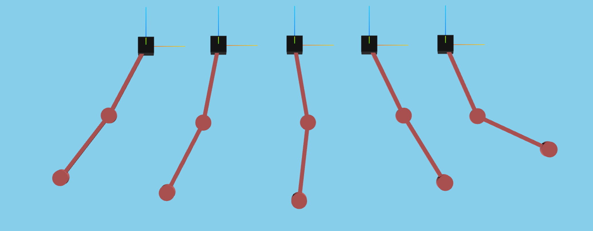
Add Visual Geometries#

We then add visual geometries to the pendulum bodies to make the simulation look nicer. These visual geometries do not affect the dynamics of the simulation and are purely for visual effect. To do this we attach Karana.Scene.ProxyScenePart bodies to our ProxyScene. We then create primitive shapes and colored materials, which we add to the first and second bodies.

# create an box geometry for the first pendulum's root attachment
box_geom = BoxGeometry(0.25, 0.25, 0.25)

# create an rectangle (box) geometry to be the pendulum arms
body_geom = BoxGeometry(0.05, 0.05, 1)

# create a cylinder geometry to be used for the end of the pendulum
cylinder_geom = CylinderGeometry(0.1, 0.1)

# create visual materials to color the bodies
mat_info = PhysicalMaterialInfo()
mat_info.color = Color.BLACK
black = PhysicalMaterial(mat_info)
mat_info.color = Color.FIREBRICK
brown = PhysicalMaterial(mat_info)
mat_info.color = Color.GOLD
gold = PhysicalMaterial(mat_info)

# attach geometry to bodies
bd1_body = ProxyScenePart("bd1_body", scene=proxy_scene, geometry=body_geom, material=brown)
bd1_body.attachTo(bd1)

bd1_pivot = ProxyScenePart("bd1_pivot", scene=proxy_scene, geometry=cylinder_geom, material=brown)
bd1_pivot.attachTo(bd1)
bd1_pivot.setTranslation([0, 0, -0.5])

bd2_body = ProxyScenePart("bd2_body", scene=proxy_scene, geometry=body_geom, material=brown)
bd2_body.setTranslation([0, 0, 0.5])
bd2_body.attachTo(bd2)

bd2_end = ProxyScenePart("bd2_end", scene=proxy_scene, geometry=cylinder_geom, material=gold)
bd2_end.attachTo(bd2)
bd2_end.setTranslation([0, 0, 0])
bd2_end.setScale(2.0)

# create an unattached object for the top of the pendulum (implicitly attached to the root frame)
root_scene_node = ProxySceneNode("root_scene_node", scene=proxy_scene)
root_part = ProxyScenePart("obstacle_part", scene=proxy_scene, geometry=box_geom, material=black)

# clean up unused variables
del (
    mat_info,
    black,
    brown,
    gold,
    bd1_body,
    bd1_pivot,
    bd2_body,
    bd2_end,
    box_geom,
    cylinder_geom,
    body_geom,
    root_scene_node,
    root_part,
)

Setup the State Propagator#

Oftentimes, a simulation consists of more than just dynamics. It may contain sensors, actuators, gravity, aerodynamics, etc. In general, we call these external interactions “models”. The Karana.Dynamics.StatePropagator provides a way to manage these models by registering and running them at the appropriate times during the Simulation.

See Models for more concepts and information.

# Set up state propagator and select integrator type: rk4 or cvode
sp = StatePropagator(mb, integrator_type=IntegratorType.RK4)

Set Initial State#

Before we begin our simulation, we set the initial state for our multibody and statepropagator.

When accessing or modifying generalized coordinates for a subhinge, it is recommended to directly set the subhinge’s values rather than for the entire multibody in order to avoid ambiguity.

# Modify the initial multibody state.
# Here we will set the first pendulum position to pi/4 radians and its velocity to 0.0
bd1.parentHinge().subhinge(0).setQ(pi / 4)
bd1.parentHinge().subhinge(0).setU(0.0)

# Initialize state. Note that in kdflex there are two states, one for multibody and one for integrator.
# Here we get the multibody state vector we updated above and then feed it to the integrator.
t_init = np.timedelta64(0, "ns")
x_init = sp.assembleState()
sp.setTime(t_init)
sp.setState(x_init)

# Syncs graphics
proxy_scene.update()

Register Models#

To simulate a model, you can either use a Karana.Dynamics.KModel or directly attach a callback function to Karana.Dynamics.StatePropagator.SpFunctions().

Here, we demonstrate using a KModel. You can implement this class yourself or use provided models like Karana.Models.UniformGravity, Karana.Models.UpdateProxyScene, and Karana.Models.SyncRealTime. Gravity must be set via a model rather than calling Karana.Dynamics.Multibody.setUniformGravAccel() once since forces are zero-ed out between derivative calls.

# Create a UniformGravity model, and set it's gravitational acceleration.
# This model contains a preDeriv method that will set the multibody's gravitational
# acceleration appropriately before each derivative call.
ug = UniformGravity("grav_model", sp, mb)
ug.params.g = np.array([0, 0, -9.81])
del ug

# by default, a change in our simulation state does not update the visualization scene.
# so we need to register a model that updates the scene after each state change.
ups = UpdateProxyScene("update_proxy_scene", sp, proxy_scene)
del ups

# typically the simulation runs as fast as possible, which is hard to visualize
# so we can use a SyncRealTime model to synchronize the simulation speed with real time.
sync_rt = SyncRealTime("sync_real_time", sp, 1.0)
del sync_rt

Register a Timed Event#

To set the length of each simulation step, we create a timed event and register it to our state propagator here. Here, we set its period to 0.1 seconds, which means our UniformGravity, UpdateProxyScene, and SyncRealTime models are also triggered every 0.1 seconds. See timed events for more information.

integrator = sp.getIntegrator()


def fn(t):
    """Print out the time and state.

    Parameters
    ----------
    t : float
        The current time.
    """
    print(f"t = {float(integrator.getTime())/1e9}s; x = {integrator.getX()}")


h = np.timedelta64(int(1e8), "ns")
t = TimedEvent("hop_size", h, fn, False)
t.period = h

# register the timed event
sp.registerTimedEvent(t)
del t

Run the Simulation#

Now, run the simulation for 10 seconds.

# print the initial state
print(f"t = {float(integrator.getTime())/1e9}s; x = {integrator.getX()}")

# run the simulation
sp.advanceTo(10.0)

# dump the state propagator info
sp.dump("sp")

t = 0.0s; x = [0.78539816 0.         0.         0.        ]
t = 0.1s; x = [ 0.76566551  0.01227844 -0.39290407  0.2433583 ]
t = 0.2s; x = [ 0.70752486  0.04776757 -0.76448294  0.45937449]
t = 0.3s; x = [ 0.61426291  0.1021731  -1.09122509  0.61593417]
t = 0.4s; x = [ 0.4916302   0.16776013 -1.34771743  0.67723754]
t = 0.5s; x = [ 0.34786321  0.23339845 -1.51055492  0.61330071]
t = 0.6s; x = [ 0.19318611  0.28582313 -1.56437937  0.4134401 ]
t = 0.7s; x = [ 0.03873567  0.31205453 -1.50690816  0.09458845]
t = 0.8s; x = [-0.10488321  0.30215441 -1.35119386 -0.30036288]
t = 0.9s; x = [-0.22912493  0.25142619 -1.12498943 -0.71120207]
t = 1.0s; x = [-0.32879004  0.16159124 -0.86631057 -1.07187795]
t = 1.1s; x = [-0.40260795  0.0406797  -0.61368587 -1.32500497]
t = 1.2s; x = [-0.4526259  -0.09871819 -0.39285307 -1.43954542]
t = 1.3s; x = [-0.48241717 -0.24276363 -0.20816994 -1.42192279]
t = 1.4s; x = [-0.49505914 -0.37983805 -0.04717697 -1.30689499]
t = 1.5s; x = [-0.49211685 -0.50221276  0.1055822  -1.13347916]
t = 1.6s; x = [-0.47395383 -0.60542956  0.25752346 -0.92615807]
t = 1.7s; x = [-0.44075037 -0.68651519  0.40492174 -0.69038419]
t = 1.8s; x = [-0.3935423  -0.74227355  0.53492008 -0.41741037]
t = 1.9s; x = [-0.3349576  -0.76824332  0.62919127 -0.09199839]
t = 2.0s; x = [-0.26955472 -0.75844362  0.6682549   0.29969942]
t = 2.1s; x = [-0.20366818 -0.70591411  0.63721559  0.76195388]
t = 2.2s; x = [-0.14455396 -0.60416481  0.53422551  1.27898084]
t = 2.3s; x = [-0.09851732 -0.44992877  0.38225298  1.79895139]
t = 2.4s; x = [-0.06783426 -0.24774197  0.23965912  2.21584788]
t = 2.5s; x = [-0.04747814 -0.01512943  0.18832901  2.38512086]
t = 2.6s; x = [-0.02539768  0.21793931  0.27497437  2.22322947]
t = 2.7s; x = [0.01094937 0.42046559 0.46165413 1.79494129]
t = 2.8s; x = [0.06747453 0.57283789 0.66514139 1.24316919]
t = 2.9s; x = [0.14228333 0.66890406 0.8193984  0.68336579]
t = 3.0s; x = [0.22864104 0.71141954 0.89359505 0.17914214]
t = 3.1s; x = [ 0.31817574  0.70751925  0.88384087 -0.24261638]
t = 3.2s; x = [ 0.4029682   0.66584522  0.80128117 -0.57665245]
t = 3.3s; x = [ 0.47656252  0.59491327  0.66276181 -0.82936327]
t = 3.4s; x = [ 0.53420211  0.50233767  0.48462532 -1.01122431]
t = 3.5s; x = [ 0.57257808  0.39475724  0.27905083 -1.13029309]
t = 3.6s; x = [ 0.58931512  0.27833935  0.05243518 -1.18737735]
t = 3.7s; x = [ 0.58240516  0.15960437 -0.19392512 -1.17485367]
t = 3.8s; x = [ 0.54985365  0.04609424 -0.46021614 -1.08114561]
t = 3.9s; x = [ 0.48981674 -0.05367644 -0.7422232  -0.9000989 ]
t = 4.0s; x = [ 0.4013204  -0.13126031 -1.02620075 -0.64043574]
t = 4.1s; x = [ 0.28530354 -0.18003065 -1.28792263 -0.32994276]
t = 4.2s; x = [ 0.1454991  -0.19700412 -1.49673544 -0.012714  ]
t = 4.3s; x = [-0.01126525 -0.18408271 -1.6226746   0.25947666]
t = 4.4s; x = [-0.17551891 -0.14819771 -1.64398809  0.44018299]
t = 4.5s; x = [-0.33627766 -0.10005889 -1.55281143  0.50230293]
t = 4.6s; x = [-0.48255899 -0.05173705 -1.35690243  0.44612043]
t = 4.7s; x = [-0.60481524 -0.01401666 -1.07627665  0.29549213]
t = 4.8s; x = [-0.69583641  0.00535715 -0.73652262  0.08503495]
t = 4.9s; x = [-0.75098827  0.00210928 -0.3628387  -0.15189707]
t = 5.0s; x = [-0.76801804 -0.02498042  0.02244076 -0.38759865]
t = 5.1s; x = [-0.74678993 -0.07454631  0.39899475 -0.59726173]
t = 5.2s; x = [-0.68919252 -0.14266965  0.74631769 -0.75393239]
t = 5.3s; x = [-0.59923468 -0.22252688  1.04249439 -0.82667971]
t = 5.4s; x = [-0.48314629 -0.30417432  1.2654361  -0.78536384]
t = 5.5s; x = [-0.34923978 -0.37509849  1.39621148 -0.61045743]
t = 5.6s; x = [-0.20740372 -0.42175725  1.42283002 -0.30200098]
t = 5.7s; x = [-0.06822974 -0.43176718  1.34383753  0.11670328]
t = 5.8s; x = [ 0.05823831 -0.39622215  1.17232622  0.59968965]
t = 5.9s; x = [ 0.1641496  -0.31186614  0.93936487  1.08038904]
t = 6.0s; x = [ 0.24563101 -0.18295009  0.69235267  1.47685119]
t = 6.1s; x = [ 0.30387058 -0.02200721  0.48173466  1.71016542]
t = 6.2s; x = [0.34422046 0.15222286 0.33619021 1.74163558]
t = 6.3s; x = [0.37302037 0.32041615 0.24645074 1.59879531]
t = 6.4s; x = [0.3942477  0.46851097 0.17877884 1.35199956]
t = 6.5s; x = [0.40845807 0.58958111 0.10231924 1.0669449 ]
t = 6.6s; x = [0.4139398  0.68187745 0.0034855  0.77996149]
t = 6.7s; x = [ 0.40849691  0.74580735 -0.11456662  0.49916143]
t = 6.8s; x = [ 0.39084982  0.78159287 -0.23765005  0.21447141]
t = 6.9s; x = [ 0.36145626  0.78795666 -0.34602247 -0.0925396 ]
t = 7.0s; x = [ 0.32283263  0.76171012 -0.41901289 -0.44034739]
t = 7.1s; x = [ 0.27940414  0.69815055 -0.44009291 -0.83929105]
t = 7.2s; x = [ 0.23675426  0.59236371 -0.40406805 -1.28121146]
t = 7.3s; x = [ 0.20000272  0.44178209 -0.3272378  -1.72451065]
t = 7.4s; x = [ 0.17113888  0.25036811 -0.25657655 -2.07883052]
t = 7.5s; x = [ 0.14615387  0.03325267 -0.26046085 -2.2187104 ]
t = 7.6s; x = [ 0.11499404 -0.18329711 -0.38169243 -2.06380435]
t = 7.7s; x = [ 0.06670038 -0.37089796 -0.59343998 -1.65574811]
t = 7.8s; x = [-0.00430109 -0.51001364 -0.82343288 -1.11491278]
t = 7.9s; x = [-0.09637788 -0.59322429 -1.00647135 -0.55284546]
t = 8.0s; x = [-0.20278086 -0.62232312 -1.1063671  -0.04151055]
t = 8.1s; x = [-0.31450582 -0.60455483 -1.11281676  0.38014768]
t = 8.2s; x = [-0.42240454 -0.54986983 -1.03161183  0.69545447]
t = 8.3s; x = [-0.5183339  -0.46909847 -0.87584982  0.90245324]
t = 8.4s; x = [-0.59557614 -0.37276507 -0.66027652  1.00840458]
t = 8.5s; x = [-0.64885128 -0.27040066 -0.39866406  1.0252103 ]
t = 8.6s; x = [-0.67417731 -0.17027737 -0.1032151   0.96561266]
t = 8.7s; x = [-0.66873634 -0.07945524  0.21480137  0.84092999]
t = 8.8s; x = [-0.63085403 -0.00393025  0.54344998  0.6614458 ]
t = 8.9s; x = [-0.56017512  0.05140568  0.8679123   0.43967649]
t = 9.0s; x = [-0.4580531   0.08321975  1.16863829  0.19501264]
t = 9.1s; x = [-0.32804707  0.09060614  1.42128165 -0.04322866]
t = 9.2s; x = [-0.17628596  0.07603581  1.59952167 -0.23771066]
t = 9.3s; x = [-0.01140046  0.04577477  1.68074317 -0.35181729]
t = 9.4s; x = [ 0.15618747  0.00916699  1.65273202 -0.36270781]
t = 9.5s; x = [ 0.31555156 -0.02328788  1.51790813 -0.27088779]
t = 9.6s; x = [ 0.45671791 -0.0423044   1.29226831 -0.09895818]
t = 9.7s; x = [ 0.57176484 -0.04152374  0.99975026  0.11928474]
t = 9.8s; x = [ 0.65528269 -0.01800637  0.66572564  0.35083831]
t = 9.9s; x = [0.70428461 0.02820962 0.31287207 0.569533  ]
t = 10.0s; x = [ 0.71786758  0.09479957 -0.03973915  0.75528156]

Clean Up the Simulation#

Below, we cleanup our simulation. We first delete local variables to remove lingering connections to objects we want to call discard on. Failing to do this will result in a use count error. We then call cleanup_graphics, a callback function returned from setupGraphics that cleans up our scene layer and webserver. This just leaves Karana.Core.discard() to cleanup any remaining Karana objects. Finally while not required, you can call Karana.Core.allDestroyed() to verify that everything is destroyed.

# Cleanup
def cleanup():
    """Cleanup the simulation."""
    global integrator, proxy_scene, web_scene, bd1, bd2
    del integrator, proxy_scene, web_scene, bd1, bd2

    discard(sp)
    cleanup_graphics()

    discard(mb)
    discard(fc)


atexit.register(cleanup)

<function __main__.cleanup()>

Summary#

Congratulations! You now understand all the fundamentals of setting up a kdFlex simulation. We covered creating a multibody, setting up a scene environment, adding visual geometries, creating a state propagator, initializing state, adding models, registering timed events, running the simulation, and cleanup.

2-link Pendulum

Contents