Flexible Slider-Crank#

This example takes the rigid slider-crank and makes one of its links flexible. Hence, this notebooks showcases a simulation that contains flexible bodies and a loop constraint.

In this example, an H5 file with the modal frequencies and mode shapes for the flexible body has already been created. This H5 file was created with FEMBridge. FEMBridge is tool available with enterprise installations of kdflex that allows one to do modal analyses on NASTRAN run decks to create H5 files like the one used here. If you do not currently have an enterprise kdflex installation, this example will not run, as FEMBridge will not be included. More information on FEMBridge will be included in an upcoming example.

Requirements:

slider-crank

In this tutorial we will:

Create the Flexible multibody using DataStruct.DataStruct
Initialize the state and constraints
Setup the kdFlex scene
Setup the state propagator and models
Run the simulation
Clean up the simulation

For a more in-depth descriptions of kdflex concepts see usage.

First, let’s verify that FEMBridge is installed

try:
    from Karana import FEMBridge
except:
    raise ModuleNotFoundError(
        "This notebook only works with an enterprise installation of kdFlex. One that includes "
        "FEMBridge. Please ensure your installation is an enterprise installation before "
        "continuing."
    )

import atexit
from numpy.typing import NDArray
import numpy as np
from copy import deepcopy
from typing import cast
from Karana.Frame import FrameContainer
from pathlib import Path
from Karana.Math import IntegratorType
from Karana.Dynamics import (
    HingeType,
    StatePropagator,
    PhysicalBody,
    SpSolverType,
    Algorithms,
)
from Karana.Dynamics.SOADyn_types import (
    BodyDS,
    HingeDS,
    PinSubhingeDS,
    BodyWithContextDS,
    MultibodyDS,
    LoopConstraintHingeDS,
    LinearSubhingeDS,
    ConstraintFrameDS,
    NodeDS,
)
from Karana.FEMBridge.ReadH5PhysicalModalBody import ReadH5PhysicalModalBody, H5PhysicalModalBodyDS
from Karana.Math import UnitQuaternion, NonlinearSolver, SolverType
from Karana.Scene import ProxyScenePart
from Karana.Scene import AssimpImporter
from Karana.Scene.Scene_types import ScenePartSpecDS
from Karana.Models import (
    UpdateProxyScene,
    ProjectConstraintError,
)
from Karana.Core import discard, allFinalized

resources = Path("../resources")

Create the Flexible Multibody#

We will create the multibody using a SOADyn_types.MultibodyDS. We begin by creating the first link.

fc = FrameContainer("root")

# Create a BodyDS for the first link. This can be used to specify all the parameters for the body, and the way
# the body attaches to it's parent, i.e., the hinge.
link_1 = BodyDS(
    name="link_1",
    mass=1.0,
    body_to_cm=np.zeros(3),
    inertia=np.eye(3),
    hinge=HingeDS(
        hinge_type=HingeType.PIN,
        subhinges=[
            PinSubhingeDS(prescribed=False, unit_axis=np.array([0.0, 1.0, 0.0]))
        ],  # pyright: ignore - Types are okay
    ),
    body_to_joint=np.array([-0.25, 0.0, 0.0]),
)

Flexible body creation#

Now, we create the second link. This is our flexible body. We use the Karana.FEMBridge.ReadH5PhysicalModalBody.ReadH5PhysicalModalBody to do so. This class reads in a Karana.FEMBridge.ReadH5PhysicalModalBody.H5PhysicalModalBodyDS instance, and creates a SOADyn_types.BodyDS instance.

hinge = deepcopy(link_1.hinge)

ds = H5PhysicalModalBodyDS(
    filename=resources / "slider_crank" / "slider_crank_beam.h5",
    p_node_grid=1,
    sensor_nodes={k: f"sn_{k}" for k in range(1, 51 + 1, 3)},
    force_nodes={},
    damping=0.2,
)
link_2_reader = ReadH5PhysicalModalBody(ds)
link_2 = link_2_reader.getModalBodyDS("link_2", hinge)
link_2.inb_to_joint = np.array([0.25, 0.0, 0.0])

link_2_context = BodyWithContextDS(body=link_2)

Now, we create the block body. This body will be attached to link_2. When we attach a body to link_2, we need to make sure that the onode of it’s joint gets the correct nodal matrix. The onode of the joint is the node attached to the parent body. Here, we are going to use the point corresponding with node 51 in the original NASTRAN run deck. The link_2_reader we created earlier has a convenience method Karana.FEMBridge.ReadH5PhysicalModalBody.ReadH5PhysicalModalBody.addInbNodeToDS for this purpose.

# We create a block body. The block is the body that will have the slider constraint,
# so we also add a constraint node via a NodeDS.
block = deepcopy(link_1)
block.name = "block"
block.mass = 1.0
block.body_to_joint = np.zeros(3)
block.constraint_nodes = [
    NodeDS(
        name="cn",
        constraint_node=True,
        force_node=True,
    )
]

# The block body is attached to link_2, so we need to use the link_2_reader to add the appropriate
# nodal matrix and inboard body to joint transform.
link_2_reader.addInbNodeToDS(block, 51)
link_2_context.children = [BodyWithContextDS(body=block, children=[])]

Now, create the rest of the MultibodyDS.

# Make link_1 prescribed
link_1.hinge.subhinges[0].prescribed = True

# Add visuals.
importer = AssimpImporter()
block_part = importer.importFrom(str(resources / "slider_crank" / "block_w_mat.glb"))
block.scene_parts = [ScenePartSpecDS.fromScenePartSpec(block_part.parts[0])]
del block_part

# Now, we combine all the bodies together to form a MultibodyDS. In addition, we add our LoopConstraint
# and a constraint frame for the slider constraint.
mbody_ds = MultibodyDS(
    name="mb",
    base_bodies=[
        BodyWithContextDS(
            body=link_1,
            children=[link_2_context],
        )
    ],
    loop_constraints=[
        LoopConstraintHingeDS(
            name="block_constraint",
            hinge=HingeDS(
                hinge_type=HingeType.SLIDER,
                subhinges=[LinearSubhingeDS(prescribed=False, unit_axis=np.array([1.0, 0.0, 0.0]))],
            ),
            get_oframe={"frame": "constraint_frame"},
            get_pframe={"body": "block", "node": "cn"},
        )
    ],
    constraint_frames=[
        ConstraintFrameDS(
            name="constraint_frame",
            translation=np.zeros(3),
            unit_quaternion=UnitQuaternion(0, 0, 0, 1),
            parent="newtonian",
        )
    ],
)

Finally, create the Multibody and cleanup any variables we don’t need.

mb = mbody_ds.toMultibody(fc)
del mbody_ds, block, link_1, link_2

Initialize the State and Constraints#

We are going to initialize the state of this system. This system contains both constraints and flexible bodies. For the constraints, we will need to use a Karana.Dynamics.ConstraintKinematicsSolver, just as we did in the rigid slider-crank example.

We could finish the state initialization here. However, when we first start moving, there may be some transient behavior, as the flexible body itself is not in the correct deformed state. Here, we create a simple equilibrium solver to deform the flexible body such that it’s initial modal coordinate acceleration is zero. In this case, the solution is trivial, as we are starting from rest, but this showcases how it can be done in general.

Satisfying the constraints#

We being by setting an initial guess for the Karana.Dynamics.ConstraintKinematicsSolver. This is done by setting all joints, body coordinates, and constraint coordinates to 0.

# Once all bodies are created, we make the Multibody current. This sets up internal
# variables for use in dynamics computations.
mb.ensureCurrent()

# Set all state data to zero
mb.resetData()
cd = mb.subhingeCoordData()

# In addition to the subhinge data, we also need to set the constraint data and body coordinate data.
cdc = mb.constraintCoordData()
cdc.setQ(0.0)
cdc.setU(0.0)
cdc.setUdot(0.0)
cdc.setT(0.0)
del cdc

bcd = mb.bodyCoordData()
bcd.setQ(0)
bcd.setU(0)
bcd.setUdot(0)
bcd.setT(0)
del bcd

Now, we use the Multibody’s ConstraintKinematicsSolver to solve for coordinates and velocities that satisfy the constraints. We want link_1’s subhinge to remain unchanged, so we freeze this coordinate. This effectively removes it from the coordinates that the ConstraintKinematicsSolver is allowed to change.

# Freeze link_1's subhinge so that the ConstraintKinematicsSolver doesn't change it.
cks = mb.cks()
cks.freezeCoord(mb.getBody("link_1").parentHinge().subhinge(0), 0)

# Now, we create a ConstraintKinematicsSolver and solve for the initial state.
errQ = cks.solveQ()
errU = cks.solveU()
del cks

# Check the errors to ensure we got a good solution.
assert abs(errQ) < 1e-6
assert abs(errU) < 1e-6

Now, let’s ensure everything is finalized.

# Before we finalize everything (see below), we need to set the gravity. In this example, there is no gravity,
# so we just set this to zero.
mb.setUniformGravAccel(np.zeros(3))

assert allFinalized()

Equilibrium#

As mentioned earlier, we solve for the flexible body’s equilibrium. Here, the solution is trivial since we are starting from rest (so the solution should be a vector of all zeros). Regardless, we include it here to showcase how solving for equilibrium can be done.

To solve for equilibrium we use a Karana.Math.NonlinearSolver. These solvers will be covered in detail in an upcoming example. For now, it is sufficient to note that they take in a function that takes in a guess for the current solution, x, and outputs values, v for that guess. The values must be modified in-place, which is why the code below uses v[:] = ... rather than v = .... Here, our equilibrium function is simple: it takes in a guess for the flexible body coordinates, q, of link_2, runs the forward dynamics, and outputs the modal accelerations of link_2. The nonlinear solver tries to drive these outputs to zero.

link_2_bd = cast(PhysicalBody, mb.getBody("link_2"))


def equilibrium(x: NDArray, v: NDArray) -> None:
    """Solve for equilibrium.

    The incoming x values will be the new Q states of the beam.
    The output v values should be the accelerations of the beam as a
    result of the incoming Q values.

    Parameters
    ----------
    x : NDArray
        New guess for beam Q values.
    v : NDArray
        Udot values of the beam after running the dynamics.
    """
    link_2_bd.setQ(x)
    Algorithms.evalForwardDynamics(mb)
    v[:] = link_2_bd.getUdot()


# Create a Nonlinear solver that uses the equilibrium function
solver = NonlinearSolver("solver", link_2_bd.nQ(), link_2_bd.nU(), equilibrium)
solver.createSolver(SolverType.HYBRID_NON_LINEAR_SOLVER)
q = np.array(link_2_bd.getQ())

# Solve for the modal coordinates that keep the modal accelerations zero
solver.solve(q)
link_2_bd.setQ(q)

Similar to the constraint solution, we can again check that the solution here is sufficient.

udot = np.empty(q.size)
equilibrium(q, udot)
assert np.linalg.norm(udot) < 1e-6

del link_2_bd
del solver

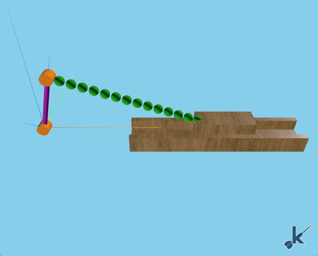
Setup the kdFlex Scene#

Here we add graphics for the scene. We will use a combination of stick parts and meshes. For the flexible body, we will use a set of sensor nodes so we can also visualize deformation.

cleanup_graphics, web_scene = mb.setupGraphics(port=0)
web_scene.defaultCamera().pointCameraAt(
    np.array([1.0, -2.0, 1.5]), np.array([1.0, 0.0, 0.0]), np.array([0.0, 0.0, 1.0])
)
del web_scene

# Add stick parts
mb.createStickParts()
scene = mb.getScene()

# Remove stick parts from the block. We added a nicer mesh when we defined the MultibodyDS
# earlier on. In addition, we remove some of the stick parts for the constraint. The linear subhinge
# for the constraint has an update function on the scene, so this must also be removed.
nd = scene.getNodesAttachedToFrame(mb.enabledConstraints()[0].hinge().pframe())[0]
scene.update_callbacks.pop("block_constraint_pframe_part_update")
discard(nd)
nd = scene.getNodesAttachedToFrame(cast(PhysicalBody, mb.getBody("block")).pnode())[0]
discard(nd)

# Rather than use the stick parts for the link_2 body, we will use a set of sensor nodes.
# These sensor nodes will deform as the flexible body itself deforms.
ndl = scene.getNodesAttachedToFrame(cast(PhysicalBody, mb.getBody("link_2")))
del scene, ndl

# Let's also add a nice mesh for the canal that the block slides in
p = importer.importFrom(str(resources / "slider_crank" / "canal_w_mat.glb")).parts[
    0
]  # pyright: ignore - importer will exist if graphics is on
part = ProxyScenePart("canal", p.geometry, mb.getScene(), p.material)
part.setTranslation(np.array([0.5 + 0.25, 0.0, 0.0]))
part.setUnitQuaternion(p.transform.getUnitQuaternion())
part.attachTo(fc.root())
del p
del part
del importer  # pyright: ignore

[WebUI] Listening at http://newton:44251

Setup the State Propagator and Models#

As in other examples, we use a Karana.Dynamics.StatePropagator to drive the simulation.

# Set up state propagator.
# Use cvode_stiff as the integrator.
sp = StatePropagator(
    mb, IntegratorType.CVODE_STIFF, None, None, SpSolverType.TREE_AUGMENTED_DYNAMICS
)

# Initialize state. Use the state from the Multibody that we set up earlier
t_init = np.timedelta64(0, "ns")
sp.setTime(t_init)
sp.setState(sp.assembleState())

# Makes sure the visualization scene is updated after each state change.
UpdateProxyScene("update_proxy_scene", sp, mb.getScene())

<Karana.Models.UpdateProxyScene at 0x7e2687857cf0>

Constraint error projection#

Even though the individual forward dynamics calls themselves should not introduce much constraint error, as we integrate, constraint error will build up. Hence, periodically, we need to use a method to eliminate this error. Here, we use the Karana.Models.ProjectConstraintError model, which uses a ConstraintKinematicsSolver to project out the error once it gets too large.

pce = ProjectConstraintError("project_error", sp, mb, sp.getIntegrator(), mb.cks())
pce.params.tol = 1e-8
h = np.timedelta64(int(1e8), "ns")
pce.setPeriod(h)
del pce

Prescribing link_1 acceleration#

Currently, our simulation won’t move, as nothing is changing the acceleration of the prescribed hinge for link_1. Here, we add a function that will modify the acceleration so that we increase the velocity for the first two seconds.

def ramp(t, _):
    """Apply prescribed Udot to move the system.

    Parameters
    ----------
    t : float
        The current time.
    _ : NDArray[np.float64]
       The current state (unused).
    """
    ft = float(t) / 1e9
    if ft < 1.0:
        u = cd.getUdot()
        u[0] = ft
        cd.setUdot(u)
    elif ft < 2.0:
        u = cd.getUdot()
        u[0] = 2.0 - ft
        cd.setUdot(u)


sp.fns.pre_deriv_fns["ramp"] = ramp

Run the Simulation#

Run the simulation for 2 revolutions.

sp.advanceTo(4 * np.pi + 1)

<SpStatusEnum.REACHED_END_TIME: 1>

Cleanup the Simulation#

Cleanup the simulation.

# Cleanup
def cleanup():
    """Cleanup the simulation."""
    global cd, link_2_context
    del cd, link_2_context
    discard(sp)
    cleanup_graphics()
    discard(mb)
    discard(fc)


atexit.register(cleanup)

<function __main__.cleanup()>

Summary#

From this tutorial you learned how to create your own flexible multibody. Additionally, you know how to set the state and constraints, solve them, and register the shock, constraint error, and acceleration models to make the simulation work.

Flexible Slider-Crank

Contents