2-link Pendulum Collision Example#
This notebook is a more advanced version of the 2-link pendulum example by adding a collision dynamics. This tutorial notebook walks you through the steps to create a 2-link pendulum manually and then adds collision dynamics in addition to extra visualization geometries.
Requirements:
In this example we will:
Create the multibody
Setup the kdFlex Scene
Setup geometries
Set up the state propagator and models
Set initial state
Register a timed event
Run the simulation
Clean up the simulation
For a more in-depth descriptions of kdflex concepts see usage.
import numpy as np
from typing import cast
import atexit
from Karana.Core import discard, BaseContainer, allFinalized
from Karana.Math import IntegratorType
from Karana.Frame import FrameContainer
from Karana.Dynamics import (
    Multibody,
    PhysicalBody,
    PhysicalBody,
    HINGE_TYPE,
    PhysicalHinge,
    PinSubhinge,
    StatePropagator,
    TimedEvent,
)
from Karana.Math import SpatialInertia, HomTran
from Karana.Scene import (
    SphereGeometry,
    BoxGeometry,
    Color,
    PhysicalMaterialInfo,
    PhysicalMaterial,
)
from Karana.Scene import ProxySceneNode, ProxyScenePart
from Karana.Scene import CoalScene
from Karana.Collision import FrameCollider, HuntCrossley
from Karana.Models import UniformGravity, UpdateProxyScene, SyncRealTime, PenaltyContact
Create the Multibody#
See Multibody or Frames for more information relating to this step.
fc = FrameContainer("root")


def createMbody():
    mb = Multibody("mb", fc)

    # inertia used for both bodies
    spI = SpatialInertia(2.0, np.zeros(3), np.diag([3, 2, 1]))

    # inboard to joint transform used for both bodies
    ib2j = HomTran()

    # body to joint transform used for both bodies
    b2j = HomTran(np.array([0, 0, 1]))

    # setup body 1
    bd1 = PhysicalBody("bd1", mb)
    bd1.setSpatialInertia(spI)
    bd1_hge = PhysicalHinge(cast(PhysicalBody, mb.virtualRoot()), bd1, HINGE_TYPE.PIN)
    bd1.setBodyToJointTransform(b2j)
    bd1_subhge = cast(PinSubhinge, bd1_hge.subhinge(0))
    bd1_subhge.setUnitAxis(np.array([0, 1, 0]))

    # setup body 2
    bd2 = PhysicalBody("bd2", mb)
    bd2.setSpatialInertia(spI)
    bd2_hge = PhysicalHinge(bd1, bd2, HINGE_TYPE.PIN)
    bd2_hge.onode().setBodyToNodeTransform(ib2j)
    bd2.setBodyToJointTransform(b2j)
    bd2_subhge = cast(PinSubhinge, bd2_hge.subhinge(0))
    bd2_subhge.setUnitAxis(np.array([0, 1, 0]))

    # finalize and verify the multibody
    mb.ensureCurrent()
    mb.resetData()
    assert allFinalized()

    return mb
mb = createMbody()

# get the first body
bd1 = mb.getBody("bd1")

# get the second body
bd2 = mb.getBody("bd2")
Setup the kdFlex Scene#
Next we setup kdflex’s graphics by calling the setupGraphics helper method on the multibody. This method takes care of setting up the graphics environment.
See Visualization and SceneLayer for more information relating to this section.
cleanup_graphics, web_scene = mb.setupGraphics(port=0, axes=0.5)

# position the viewpoint camera of the visualization
web_scene.defaultCamera().pointCameraAt([0.4, 4, -0.9], [0, 0, -1], [0, 0, 1])
proxy_scene = mb.getScene()
[WebUI] Listening at http://newton:35339
To our SceneLayer, we register a Karana.Scene.CoalScene instance to perform collision and distance queries using the geometries populated in Karana.Scene.ProxyScene. CoalScene is a wrapper of the open source Coal project.
See Collisions for more information.
col_scene = CoalScene("collision_scene")
proxy_scene.registerClientScene(col_scene, mb.virtualRoot())
Setup Geometries#
We create 3d geometries with associated material properties and attach them to bodies. This is commonly useful for collision detection and 3d visualization.
# create a ball geometry to be used for both bodies
ball_geom = SphereGeometry(0.1)

# create an obstacle geometry to be placed in the path of body 2
obstacle_geom = BoxGeometry(0.2, 0.2, 0.2)

# create red and blue visualize materials to color the bodies
mat_info = PhysicalMaterialInfo()
mat_info.color = Color.BLUE
blue = PhysicalMaterial(mat_info)
mat_info.color = Color.RED
red = PhysicalMaterial(mat_info)

# create a ProxyScenePart and attach it to the body
bd1_part = ProxyScenePart("bd1_part", scene=proxy_scene, geometry=ball_geom, material=blue)
bd1_part.attachTo(bd1)

bd2_part = ProxyScenePart("bd2_part", scene=proxy_scene, geometry=ball_geom, material=blue)
bd2_part.attachTo(bd2)
Now, we create a separate obstacle for the 2nd pendulum link to collide with. Since it is separate from the pendulum, it is attached to the root frame.
# create some unattached objects (implictly attached to the root frame)
root_scene_node = ProxySceneNode("root_scene_node", scene=proxy_scene)
obstacle_part = ProxyScenePart("obstacle_part", scene=proxy_scene, geometry=obstacle_geom)
obstacle_part.setTranslation([0.1, 0, -2])

del obstacle_geom, mat_info, ball_geom
For visual effects, we visualize the axes for the root, body 1, and body 2. Additionally, we add a trail following the motion of body 2.
# visualize axes for important frames
root_scene_node.graphics().showAxes(0.5)
bd1_part.graphics().showAxes(0.5)
bd2_part.graphics().showAxes(0.5)

# add a trail to track the motion of body 2
bd2_part.graphics().trail()

proxy_scene.update()
Setup State Propagator and Models#
Now, we setup the Karana.Dynamics.StatePropagator and register our models as well.
See Models for more concepts and information.
# set up state propagator
sp = StatePropagator(mb, IntegratorType.CVODE)
integ = sp.getIntegrator()
sp_options = sp.getOptions()

# Create a UniformGravity model, and set it's gravitational acceleration.
ug = UniformGravity("grav_model", sp, mb)
ug.params.g = np.array([0, 0, -9.81])
del ug

# Makes sure the visualization scene is updated after each state change.
UpdateProxyScene("update_proxy_scene", sp, proxy_scene)

# sync the simulation time with real-time.
SyncRealTime("sync_real_time", sp, 1.0)
Because our CoalScene managed distance queries and collision detection, we now attach a Karana.Models.PenaltyContact using the CoalScene and ProxyScene to apply counter forces whenever registered bodies collide.
# Set penalty contact model parameters
hc = HuntCrossley("hunt_crossley_contact")
hc.params.kp = 100000
hc.params.kc = 10000
hc.params.mu = 0.3
hc.params.n = 1.5
hc.params.linear_region_tol = 1e-3

PenaltyContact("penalty_contact", sp, mb, [FrameCollider(proxy_scene, col_scene)], hc)

del hc
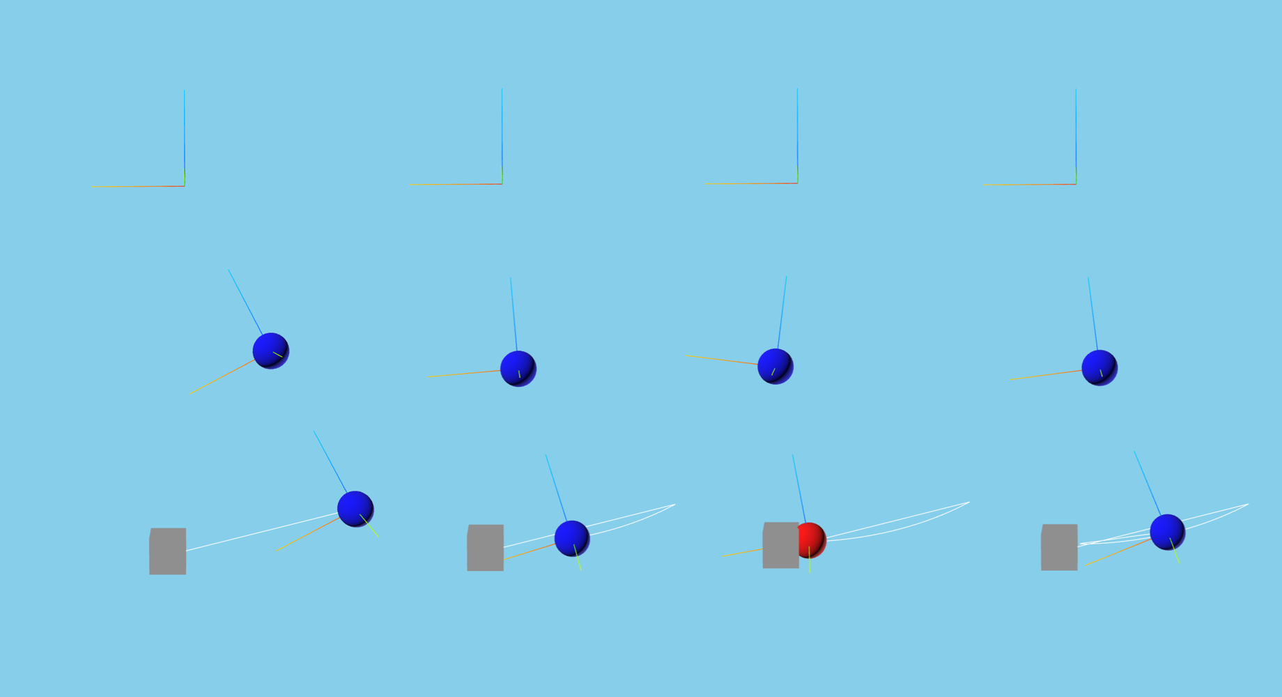
Now we register a callback function that is run at the end of each timestep. It directly queries for if body 2 is in collision with the obstacle, and turns body 2 red if so.
def post_step_fn(t, x):
    if bd2_part.collision().collide(obstacle_part.collision()):
        bd2_part.setMaterial(red)
    else:
        bd2_part.setMaterial(blue)


sp_options.fns.post_hop_fns["update_and_info"] = post_step_fn
Set Initial State#
Before we begin our simulation, we set the initial state for our multibody and statepropagator.
When accessing or modifying generalized coordinates for a subhinge, it is recommended to directly set the subhinge’s values rather than for the entire multibody in order to avoid ambiguity.
# Modify the initial multibody state.
# Here we will set the first pendulum position to 0.5 radians and its velocity to 0.0
bd1 = mb.getBody("bd1")
bd1.parentHinge().subhinge(0).setQ([0.5])
bd1.parentHinge().subhinge(0).setU([0.0])

# set integrator state
t_init = np.timedelta64(0, "ns")
x_init = mb.dynamicsToState()
sp.setTime(t_init)
sp.setState(x_init)

# Syncs up graphics
proxy_scene.update()
Register a Timed Event#
Because the penalty contact model applies forces proportional to the overlap between two objects in collision, it is necessary to shorten the period. Otherwise, if a collision is only detected when 2 objects have significant overlap, unrealistic forces may be applied.
h = np.timedelta64(int(1e7), "ns")
t = TimedEvent("hop_size", h, lambda _: None, False)
t.period = h

# register after time has been initialized
sp.registerTimedEvent(t)
del t
Run the Simulation#
Karana.Math.Integrator.advanceTo() can be increased to lengthen the simulation
# print the initial state
print(f"t = {float(integ.getTime())/1e9}s; x = {integ.getX()}")

# run the simulation
sp.advanceTo(10.0)
t = 0.0s; x = [0.5 0. 0. 0. ]
<SpStatusEnum.REACHED_END_TIME: 1>
Clean Up the Simulation#
Below, we cleanup our simulation. We first delete local variables, cleanup our visualizer, discard remaining Karana objects, and optionally verify using allDestroyed.
def cleanup():
    global sp_options, integ, proxy_scene, web_scene, col_scene
    global root_scene_node, bd1, bd2, obstacle_part, red, blue, bd1_part, bd2_part
    del (
        sp_options,
        integ,
        proxy_scene,
        web_scene,
        col_scene,
        root_scene_node,
        bd1,
        bd2,
        obstacle_part,
        red,
        blue,
        bd1_part,
        bd2_part,
    )

    discard(sp)
    cleanup_graphics()

    discard(mb)
    discard(fc)

    bc = BaseContainer.singleton()
    bc.at_exit_fns.executeReverse()
    bc.at_exit_fns.clear()
    del bc


atexit.register(cleanup)
<function __main__.cleanup()>
Summary#
You now know how to setup a 2-link pendulum with a obstacle to simulate collisions. By attaching a CoalScene and creating a PenaltyContact model, the simulation is able to model collisions.
Further Readings#
Simulate collisions with a n-link pendulum
Drive an ATRVjr rover