Import/Export Multibodies#
In this notebook we demonstrate how to export and import kdflex multibodies to various formats. This notebook follows almost the same procedure as the \(n\)-body pendulum notebook, but differs in that it demonstrates how to export a multibody after it has been created as well as how to import one. Everything included after the import cell in this notebook has already been demonstrated in other notebooks, and has only been included to prove that the imported multibody can now be ran. As such feel free to skip the rest of the notebook after that section.
Requirements:
In this tutorial we will:
Create the multibody
Export/Import the multibody
Setup the kdFlex Scene
Add a root visual geometry
Set up the state propagator and models
Set initial state
Register a timed event
Run the simulation
Clean up the simulation
For a more in-depth descriptions of kdflex concepts see usage.
import numpy as np
import atexit
from typing import cast
from math import pi
from Karana.Core import discard, allReady
from Karana.Frame import FrameContainer
from Karana.Math import IntegratorType
from Karana.Dynamics import (
    Multibody,
    PhysicalBody,
    PhysicalBody,
    HingeType,
    StatePropagator,
    TimedEvent,
    PhysicalBodyParams,
)
from Karana.Math import SpatialInertia, HomTran
from Karana.Models import Gravity, UniformGravity, UpdateProxyScene, SyncRealTime, OutputUpdateType
from Karana.Scene import (
    BoxGeometry,
    CylinderGeometry,
    Color,
    PhysicalMaterialInfo,
    PhysicalMaterial,
    ScenePartSpec,
)
from Karana.Dynamics.SOADyn_types import MultibodyDS
Create the Multibody#
Below we create the 2-link pendulum that we will export in different formats. We are using the procedural approach since it is simpler and we can build the multibody and add visual parts all at once. If you would like to learn more about the procedural approach, check out the n-link Pendulum example.
See Multibody or Frames for more information relating to this step.
fc = FrameContainer("root")


def createMbody(n_links: int):
    """Create the multibody.

    Parameters
    ----------
    n_links : int
        The number of pendulum links to use.
    """
    mb = Multibody("mb", fc)

    # create visual materials to color the bodies
    mat_info = PhysicalMaterialInfo()
    mat_info.color = Color.FIREBRICK
    brown = PhysicalMaterial(mat_info)

    # using scene part spec to define visual geometry for each procedural body
    sp_body = ScenePartSpec()
    sp_body.name = "sp0"
    sp_body.geometry = BoxGeometry(0.05, 0.05, 1)
    sp_body.material = brown
    sp_body.transform = HomTran([0.0, 0.0, 0.0])
    sp_body.scale = [1, 1, 1]

    sp_pivot = ScenePartSpec()
    sp_pivot.name = "sp1"
    sp_pivot.geometry = CylinderGeometry(0.1, 0.1)
    sp_pivot.material = brown
    sp_pivot.transform = HomTran([0.0, 0.0, -0.5])
    sp_pivot.scale = [1, 1, 1]

    # Here, we use the addSerialChain method to add multiple instances of the same body
    # connected in a chain. We add n instances of the pendulum link with the following parameters:
    params = PhysicalBodyParams(
        spI=SpatialInertia(2.0, np.zeros(3), np.diag([3, 2, 1])),
        axes=[np.array([0.0, 1.0, 0.0])],
        body_to_joint_transform=HomTran(np.array([0, 0, 0.5])),
        inb_to_joint_transform=HomTran(np.array([0, 0, -0.5])),
        scene_part_specs=[sp_body, sp_pivot],
    )
    PhysicalBody.addSerialChain(
        "link",
        n_links,
        cast(PhysicalBody, mb.virtualRoot()),
        htype=HingeType.REVOLUTE,
        params=params,
    )

    # finalize and verify the multibody
    mb.ensureHealthy()
    mb.resetData()
    assert allReady()

    return mb
We then create the multibody by calling the createMbody method we defined in the previous cell.
# initialization
n_links = 2
mb = createMbody(n_links)
Export/Import the Multibody#
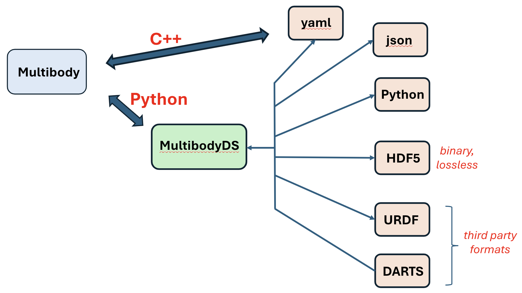
Now that we have the multibody we convert it from a Karana.Dynamics.Multibody to a intermediate Karana.Dynamics.SOADyn_types.MultibodyDS DataStruct type, which we then export to various file formats.
See Model Data Files for more info.
mb_DS_to_export = mb.toDS()

# delete old multibody
discard(mb)

# export to JSON
mb_DS_to_export.toFile("2_link_multibody.json")

# export multibody to yaml
mb_DS_to_export.toFile("2_link_multibody.yaml")

# export multibody to hdf5
mb_DS_to_export.toFile("2_link_multibody.hdf5")
We now import the exported Karana.Dynamics.SOADyn_types.MultibodyDS Multibody DataStruct. After importing we convert it back to a Karana.Dynamics.Multibody. We have to run the Karana.Core.LockingBase.ensureHealthy() and Karana.Dynamics.SubTree.resetData() methods after we import a model even if the initial model we exported had these methods ran. After this point, the multibody should be functionally identical to the original multibody we defined procedurally with the createMBody() method above. Since the multibody is identical, the notebook from this point is the same as the \(n\)-link pendulum, since it is the same exact process to run the simulation. You can run the rest of the notebook if you would like, but there will be no new concepts introduced after the following cell.
imported_ds = MultibodyDS.fromFile("2_link_multibody.json")
# imported_ds = MultibodyDS.fromFile("2_link_multibody.yaml")
# imported_ds = MultibodyDS.fromFile("2_link_multibody.hdf5")

mb_new = imported_ds.toMultibody(fc)

# Even if a multibody is reimported we have to use ensureHealthy() to make sure
# the multibody is healthy. We then also can use resetData() to initialize the
# state and set coordinates at zero.
mb_new.ensureHealthy()
mb_new.resetData()

# verify that the imported multibody is ready to go
assert allReady()

mb_new.dumpTree()
|-mb_MBVROOT_
   |-link_0
      |-link_1
Setup the kdFlex Scene#
Next we setup kdflex’s graphics by calling the setupGraphics helper method on the multibody. This method takes care of setting up the graphics environment.
See Visualization and Scene Layer for more information relating to this section.
cleanup_graphics, web_scene = mb_new.setupGraphics(port=0, axes=0.0)

# position the viewpoint camera of the visualization
web_scene.defaultCamera().pointCameraAt([0.0, 5.0, -1.0], [0, 0, -1], [0, 0, 1])

# Get the scene for later use
proxy_scene = mb_new.getScene()
[WebUI] Listening at http://newton:34183
Setup State Propagator and Models#
Now, we setup the Karana.Dynamics.StatePropagator and register our models as well.
See Models for more concepts and information.
# Set up state propagator and select integrator type: rk4 or cvode
sp = StatePropagator(mb_new, integrator_type=IntegratorType.RK4)
integrator = sp.getIntegrator()

# add a gravitational model to the state propagator
ug = Gravity("grav_model", sp, UniformGravity("uniform_gravity"), mb_new)
ug.getGravityInterface().setGravity(np.array([0, 0, -9.81]), 0.0, OutputUpdateType.PRE_HOP)
del ug

# Makes sure the visualization scene is updated after each state change.
UpdateProxyScene("update_proxy_scene", sp, proxy_scene)

# sync the simulation time with real-time.
SyncRealTime("sync_real_time", sp, 1.0)


# Register a post step function to log state information.
def post_step_fn(t, x):
    """Print out the time and state.

    Parameters
    ----------
    t : float
        The current time.
    x : NDArray[np.float64]
       The current state.
    """
    print(f"t = {float(integrator.getTime())/1e9}s; x = {integrator.getX()}")


sp.fns.post_hop_fns["update_and_info"] = post_step_fn
Set Initial State#
Before we begin our simulation, we set the initial state for our multibody and statepropagator.
When accessing or modifying generalized coordinates for a subhinge, it is recommended to directly set the subhinge’s values rather than for the entire multibody in order to avoid ambiguity.
# Initialize the multibody state.
# Here we will set the first pendulum position to pi/8 radians and its velocity to 0.0
bd1 = mb_new.getBody("link_0")
bd1.parentHinge().subhinge(0).setQ(pi / 4)
bd1.parentHinge().subhinge(0).setU(0.0)

# Initialize the integrator state
t_init = np.timedelta64(0, "ns")
x_init = sp.assembleState()
sp.setTime(t_init)
sp.setState(x_init)

# Syncs graphics
proxy_scene.update()
Register a Timed Event#
To terminate a simulation step every 0.1 seconds, we create a timed event and register it to our state propagator here. See timed events for more information.
h = np.timedelta64(int(1e8), "ns")
t = TimedEvent("hop_size", h, lambda _: None, False)
t.period = h

# register the timed event
sp.registerTimedEvent(t)
del t
Run the Simulation#
Now, run the simulation for 10 seconds.
# run the simulation
print(f"t = {float(integrator.getTime())/1e9}s; x = {integrator.getX()}")

# run the simulation
sp.advanceTo(10.0)

# dump the state propagator info
sp.dump("sp")
t = 0.0s; x = [0.78539816 0.         0.         0.        ]
t = 0.1s; x = [ 0.76349445  0.01680313 -0.43624439  0.33371087]
t = 0.2s; x = [ 0.69888834  0.06577862 -0.85022684  0.63827478]
t = 0.3s; x = [ 0.59499828  0.14234329 -1.21770063  0.87926231]
t = 0.4s; x = [ 0.45777804  0.23818444 -1.51246493  1.01726067]
t = 0.5s; x = [ 0.29578038  0.34113369 -1.70949023  1.01662179]
t = 0.6s; x = [ 0.11978697  0.43621738 -1.79010604  0.85901723]
t = 0.7s; x = [-0.05806892  0.50791391 -1.74649608  0.5524414 ]
t = 0.8s; x = [-0.22550436  0.54277735 -1.58356094  0.1292049 ]
t = 0.9s; x = [-0.37134283  0.53138927 -1.31825157 -0.36444363]
t = 1.0s; x = [-0.48660819  0.46916797 -0.97709001 -0.87959775]
t = 1.1s; x = [-0.56530097  0.35624875 -0.59239322 -1.37145346]
t = 1.2s; x = [-0.60476258  0.19697353 -0.19794044 -1.80056533]
t = 1.3s; x = [-6.05605290e-01 -5.91349616e-04  1.75352580e-01 -2.13186132e+00]
t = 1.4s; x = [-0.5712026  -0.22516493  0.503928   -2.33699369]
t = 1.5s; x = [-0.50674337 -0.46326313  0.77544607 -2.40147497]
t = 1.6s; x = [-0.41807229 -0.70085943  0.98857346 -2.32882141]
t = 1.7s; x = [-0.31085454 -0.9249631   1.14692464 -2.13456555]
t = 1.8s; x = [-0.19047512 -1.12428471  1.2514652  -1.8356949 ]
t = 1.9s; x = [-0.06252719 -1.28904021  1.29693848 -1.44499766]
t = 2.0s; x = [ 0.06661033 -1.41052612  1.27347608 -0.97170898]
t = 2.1s; x = [ 0.18952507 -1.48090589  1.17108931 -0.42437044]
t = 2.2s; x = [ 0.29799175 -1.49324731  0.98411517  0.18731851]
t = 2.3s; x = [ 0.38355233 -1.44165895  0.7138203   0.85230024]
t = 2.4s; x = [ 0.4382625  -1.32140652  0.36930346  1.5584436 ]
t = 2.5s; x = [ 0.45551223 -1.12909132 -0.03154281  2.29026962]
t = 2.6s; x = [ 0.43105868 -0.86344568 -0.45819652  3.01739087]
t = 2.7s; x = [ 0.3647267  -0.52815106 -0.85781785  3.66491659]
t = 2.8s; x = [ 0.2631527  -0.13805693 -1.14795373  4.08412802]
t = 2.9s; x = [ 0.14148259  0.27561166 -1.25245558  4.12092901]
t = 3.0s; x = [ 0.01876834  0.67347749 -1.17801964  3.78700418]
t = 3.1s; x = [-0.09076816  1.02611299 -1.00267344  3.24520398]
t = 3.2s; x = [-0.18070413  1.32041526 -0.79393106  2.63699632]
t = 3.3s; x = [-0.24948606  1.55350894 -0.58228958  2.02686807]
t = 3.4s; x = [-0.29735189  1.72635962 -0.3760869   1.43321122]
t = 3.5s; x = [-0.32491508  1.84073783 -0.17623962  0.8569881 ]
t = 3.6s; x = [-0.33282077  1.89820988  0.01691665  0.29432755]
t = 3.7s; x = [-0.3218028   1.89989899  0.20192701 -0.25945707]
t = 3.8s; x = [-0.29276814  1.84645748  0.37702139 -0.80907413]
t = 3.9s; x = [-0.24674969  1.73806518  0.54170318 -1.35924757]
t = 4.0s; x = [-0.18471938  1.57444845  0.69770882 -1.91407647]
t = 4.1s; x = [-0.10740371  1.35506757  0.84768945 -2.47387501]
t = 4.2s; x = [-0.01543271  1.07989354  0.98947492 -3.02570296]
t = 4.3s; x = [ 0.08962705  0.7516833   1.10403725 -3.5222507 ]
t = 4.4s; x = [ 0.20284524  0.38081495  1.14188599 -3.8559983 ]
t = 4.5s; x = [ 0.31310333 -0.00917991  1.03517073 -3.88477861]
t = 4.6s; x = [ 0.40406363 -0.38397644  0.75852058 -3.55757752]
t = 4.7s; x = [ 0.46077951 -0.71213102  0.36268605 -2.97570687]
t = 4.8s; x = [ 0.47522711 -0.97530943 -0.07501427 -2.2773575 ]
t = 4.9s; x = [ 0.44640263 -1.166667   -0.49479514 -1.54918461]
t = 5.0s; x = [ 0.37817678 -1.28559619 -0.85799031 -0.83384591]
t = 5.1s; x = [ 0.27751426 -1.33470554 -1.14051932 -0.15638146]
t = 5.2s; x = [ 0.15321121 -1.31882116 -1.32952956  0.46279   ]
t = 5.3s; x = [ 0.0148421  -1.24472448 -1.42210371  1.00491175]
t = 5.4s; x = [-0.12815369 -1.12097104 -1.42341636  1.45340278]
t = 5.5s; x = [-0.26711511 -0.95763683 -1.34314207  1.79447311]
t = 5.6s; x = [-0.39438612 -0.76604025 -1.19103905  2.0170366 ]
t = 5.7s; x = [-0.50316135 -0.55846602 -0.97417133  2.11305241]
t = 5.8s; x = [-0.58722342 -0.34776126 -0.69765199  2.07986976]
t = 5.9s; x = [-0.64091309 -0.1466203  -0.3681918   1.92363902]
t = 6.0s; x = [-0.65947136  0.03336685  0.00253218  1.66003575]
t = 6.1s; x = [-0.63960824  0.18252551  0.39682845  1.31100668]
t = 6.2s; x = [-0.58007869  0.29354182  0.79165304  0.90157381]
t = 6.3s; x = [-0.48216446  0.361769    1.15973107  0.46047252]
t = 6.4s; x = [-0.35001818  0.385752    1.47131517  0.02327514]
t = 6.5s; x = [-0.19076578  0.36800047  1.69733992 -0.36654687]
t = 6.6s; x = [-0.01422113  0.31559233  1.81392059 -0.66249057]
t = 6.7s; x = [ 0.16787659  0.23995321  1.80717068 -0.82630933]
t = 6.8s; x = [ 0.34305552  0.15536257  1.6766659  -0.84096689]
t = 6.9s; x = [ 0.49949913  0.07644337  1.43561452 -0.71662844]
t = 7.0s; x = [ 0.62724411  0.01565407  1.10696882 -0.48454749]
t = 7.1s; x = [ 0.71885836 -0.01816522  0.717433   -0.18357692]
t = 7.2s; x = [ 0.76955857 -0.01995339  0.29274385  0.15072578]
t = 7.3s; x = [ 0.77700883  0.01210616 -0.14388367  0.48880448]
t = 7.4s; x = [ 0.74111058  0.07701767 -0.57058868  0.80297933]
t = 7.5s; x = [ 0.66397465  0.17085427 -0.9647299   1.06150285]
t = 7.6s; x = [ 0.55006771  0.28619662 -1.30185487  1.22654793]
t = 7.7s; x = [ 0.40633936  0.41175208 -1.55723601  1.2601306 ]
t = 7.8s; x = [ 0.24207356  0.53292702 -1.70959971  1.13636458]
t = 7.9s; x = [ 0.06834581  0.63361776 -1.7449035   0.85204611]
t = 8.0s; x = [-0.10282791  0.69864429 -1.65865107  0.42830333]
t = 8.1s; x = [-0.25951365  0.71589169 -1.45713524 -0.09621135]
t = 8.2s; x = [-0.39097389  0.67758522 -1.15798998 -0.67481945]
t = 8.3s; x = [-0.4887746   0.58070844 -0.78935903 -1.25980126]
t = 8.4s; x = [-0.54771921  0.42696819 -0.38728864 -1.80429435]
t = 8.5s; x = [-0.5664483   0.22280248  0.00833045 -2.26015922]
t = 8.6s; x = [-0.54753787 -0.02047007  0.36000742 -2.57897001]
t = 8.7s; x = [-0.49679459 -0.28718633  0.64238126 -2.72551941]
t = 8.8s; x = [-0.42157046 -0.55966837  0.8504973  -2.69686178]
t = 8.9s; x = [-0.32878829 -0.82165355  0.99610191 -2.52181486]
t = 9.0s; x = [-0.22394984 -1.06042353  1.09343767 -2.23829524]
t = 9.1s; x = [-0.11150521 -1.26664066  1.14828597 -1.87418954]
t = 9.2s; x = [ 0.00415919 -1.43306968  1.15654672 -1.44412297]
t = 9.3s; x = [ 0.11793123 -1.55348667  1.10874978 -0.95472389]
t = 9.4s; x = [ 0.22372184 -1.62216616  0.99566363 -0.41002101]
t = 9.5s; x = [ 0.31470488 -1.63378167  0.8122178   0.1857907 ]
t = 9.6s; x = [ 0.38382486 -1.5834643   0.5589675   0.8277682 ]
t = 9.7s; x = [ 0.42436188 -1.46686629  0.2420341   1.51042091]
t = 9.8s; x = [ 0.43049312 -1.28025655 -0.1265392   2.22629459]
t = 9.9s; x = [ 0.39801312 -1.02104997 -0.52545576  2.95735211]
t = 10.0s; x = [ 0.3256916  -0.68999641 -0.91411491  3.6485481 ]
sp |---> Dumping "sp"  ({py:class}`Karana.Core.LockingBase`)
sp <Base> id=806
sp <Base> refCount=1
sp <LockingBase> isHealthy=true
sp <LockingBase> upstream deps:
sp <LockingBase> downstream deps:
sp Dumping StatePropagator:   time=10s, nstates=4, integrator=RK4
sp    pre hop fns:
sp       Dumping functions in callback registry:
sp       	0: sync_real_time_pre_hop
sp    pre deriv fns:
sp       Dumping functions in callback registry:
sp       	0: grav_model
sp    post hop fns:
sp       Dumping functions in callback registry:
sp       	0: update_proxy_scene_post_hop
sp       	1: sync_real_time_post_hop
sp       	2: update_and_info
sp        Dumping scheduler: num_before_hop_timed_events 0, num_after_hop_timed_events 1
sp            Before hop events:
sp            After hop events:
sp              Dumping TimedEvent hop_size
sp                 Has event set.
sp                 Next scheduled event time: 10100000000ns
sp                 This will run after the hop.
sp                 Will be rescheduled with a period of 100000000ns.
sp                 Has a priority of 0.
sp    Counters: hops=100, derivs=400, integration steps=100, zero crossings=0
Clean Up the Simulation#
Below, we cleanup our simulation. We first delete local variables, cleanup our visualizer, discard remaining Karana objects, and optionally verify using allDestroyed.
# Cleanup
def cleanup():
    """Cleanup the simulation."""
    global integrator, mb_DS_to_export, proxy_scene, web_scene, imported_ds, bd1
    del integrator, mb_DS_to_export, proxy_scene, web_scene, imported_ds, bd1
    discard(sp)
    cleanup_graphics()
    discard(mb_new)
    discard(fc)


atexit.register(cleanup)
<function __main__.cleanup()>
Summary#
By converting between Karana.Dynamics.SOADyn_types.MultibodyDS and Karana.Dynamics.Multibody for both import and export, you are able to load multibodies from files and save them into files. This opens up many exciting possibilities!
Further Readings#
Load a mars 2020 rover urdf
Load a robotic arm urdf
Enforce loop constraints in a double-wishbone model
Create and use constraints in a slider-crank model
Drive an ATRVjr rover