Reference Guide#
Basics#
C++ and Python layers#
The core software for kdFlex is in C++ (C++20 standard) and uses an
object-oriented design. Additionally Python bindings that mirror the
C++ API are available as well. The feature complete Python
bindings provide an excellent avenue for developing and prototyping
simulation software. The Python interface is especially useful for scripting,
interacting with the simulation and introspection of the simulation
content. This combination of languages provides a best-of-both-worlds,
where users can setup and introspect their simulation using Python while
obtaining the high performance of compiled C++.
The C++ object public interfaces are mirrored at
the Python level and can be used for scripting and interacting with
the software. The Python modules are included in the Karana Python
package.
Simulations are not required to use Python at all, and can be written entirely in
C++ if desired. When using the C++ API, it is recommended that users build with cmake,
as this provides the simplest way to compile/link code correctly. A sample CMakeLists.txt
file is provided below.
# CMakeLists.txt for building script.cpp
cmake_minimum_required(VERSION 3.25)
project(my_project)

# Find the Karana package
set(Eigen3_DIR /path/to/eigen3/cmake/files) # This should be eigen 5.0
find_package(Karana REQUIRED)

# Optional: Enable compile commands. This is used by LSPs.
set(CMAKE_EXPORT_COMPILE_COMMANDS ON)

# Example binary
add_executable(my_bin main.cc)
target_link_libraries(1_link Karana::kdflex)
It is important to note that the version of Eigen used is 5.0.0. Most package
managers have a version of Eigen that is outdated by a few years and is missing critical bug fixes.
Users should clone the Eigen package at this commit using
git clone --depth 1 --branch 5.0.0 --single-branch https://gitlab.com/libeigen/eigen.git eigen_5.0.0
The package can be built and installed using cmake. For example, by using
cmake -DCMAKE_INSTALL_PREFIX=/path/to/desired/install/dir -B build .
cd build
make install -j 10
After installation, the Eigen cmake files will be available at the installed location under share/eigen3/cmake.
Of course, C++ applications can be built without cmake if desired. When doing so, users will need to
include the header files in /usr/include/Karana and link against libkdflex.so in /usr/lib. In addition, they
will need to include headers for Eigen (again, these need to be the header files of Eigen 5.0) and spdlog,
as well as link against libspdlog and the libfmt libraries.
Furthermore, they will need to use the following compiler flags: -DFMT_SHARED -DSPDLOG_COMPILED_LIB -DSPDLOG_FMT_EXTERNAL -DSPDLOG_SHARED_LIB -std=gnu++20 -msse -msse2 -mssse3 -msse4.1 -msse4.2 -mavx -mavx2.
Creating and discarding objects#
The general convention in kdFlex is to use create() static factory
methods to create new instances of objects - instead of calling the
constructor. Virtually all of the classes have implementations of this
method. So to create an instance of class A call the static
A::create() method. On the other hand, to discard an object instance
you just need to call the object’s obj->discard() method (instead of
calling the destructor). Thus an instance of the
Karana.Dynamics.PhysicalBody can be created by calling
Karana.Dynamics.PhysicalBody.create() method, and can be discarded
by calling the Karana.Core.discard() method.
Usage tracking of objects#
kdFlex supports configuration changes to the system to support the
simulation of complex scenarios where multibody systems can undergo
topological changes from the creation and removal of bodies, nodes,
hinges etc. kdFlex uses shared pointers and their associated
reference counting to avoid use after free errors. However, this is
not sufficient since having dependencies linger past the stage where the
object is no longer supposed to exist introduces vulnerabilities.
kdFlex implements more rigorous usage tracking that requires all
dependencies on an object to have been removed before the object can be
discarded. Enforcement of such strict housekeeping can take a little
get used to, but helps ensure that complex configuration changes can be
carried out robustly at run-time within simulations. Such usage tracking
is applied at both the C++ and Python levels. The example
simulations such as 2 link pendulum (basic) include a
cleanup section at the end where objects are explicitly discarded to
ensure clean shutdown at the end of a simulation.
In the event that a user runs into issues discarding objects and cannot find a way forward, assistance from a Karana employee is always available via the forum or tickets system. However, in the case that a user must move forward immediately and cannot wait for assistance, the Karana.Core.DebugManager.enable_usage_tracking_map_errors can be used to disable usage tracking: see the DebugManager section for details.
The dump() method#
Most kdFlex classes implement specializations of the
Karana.Core.Base.dump() method. This method can be used for
introspection to display useful information specifically about an object
instance.
Math layer#
kdFlex builds on the Eigen math library
basic classes, and extends and sub-classes them as needed. The derived
classes are available under the Karana::Math namespace. The
Karana::Math::Vec, Karana::Math::Vec3, Karana::Math::Mat,
Karana::Math::Mat33 etc are simple aliases around the basic Eigen
array classes.
While vectors are matrices at the C++ level correspond to the Eigen
classes, their corresponding Python equivalents are numpy
arrays. Methods that take and return Eigen arrays at the C++ level,
take and return numpy arrays at the Python level. This by far is the
largest difference between the C++ and Python APIs. Otherwise, with
few exceptions, the Python methods consistently replicate the C++ class
and method interfaces.
The Math layer also defines a special NaN value, Karana::Math::notReadyNaN, for use in places where a numerical variable is needed but its value is has not yet been initialized. The function Karana::Math::isNotReadyNaN() checks if a given number has this special value. When not ready, the math objects in kdFlex will be populated with this special value to avoid undefined behavior or confusion with NaNs resulting from bad numerics.
Frames Layer#
Pose representations#
kdFlex supports a number of types of attitude representations
including Karana.Math.RotationMatrix for direction cosine rotation
matrices, Karana.Math.RotationVector for rotation vectors, and
Karana.Math.UnitQuaternion for unit quaternions. The
Karana.Math.EulerAngles attitude representation at the Python
level and Eigen::AngleAxis and Eigen::EulerAngles attitude representations
at the C++ level are also available for use. Unit quaternions are the ones used
most broadly in kdFlex since they are free of singularities and
computationally more efficient. Methods are available to transform
between these different representations. While unit quaternions keep the
vector and scalar components separately, in cases where they are
combined, the convention is to keep the scalar component last after the
vector elements.
kdFlex uses the passive approach for attitude representations. Thus the product \({}^a v = {}^a R_b {}^b v\) denotes the conversion of the the coordinates of the \(v\) vector from the \(b\) frame to the \(a\) frame.
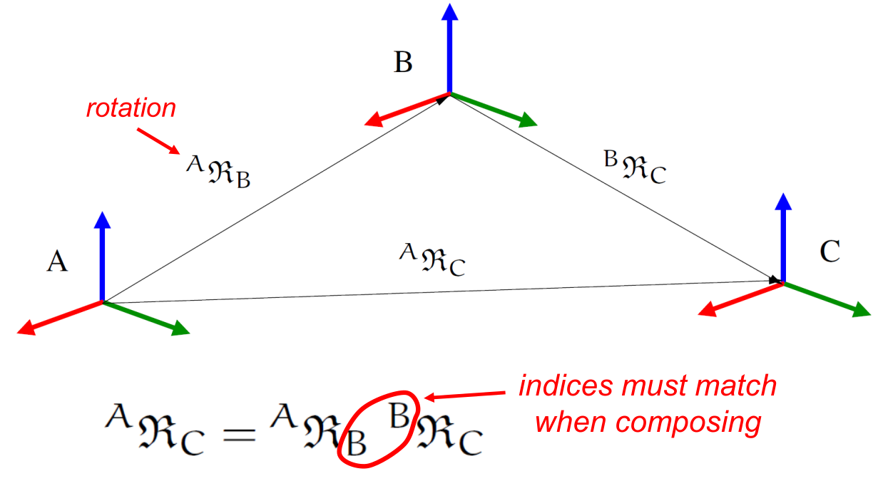
Accumulation of rotations across frames#
Since unit quaternions are not a minimal attitude representation, the
minimal coordinate rotation vector attitude representations
are used instead as coordinates when parameterizing the relative
attitude for Karana.Dynamics.SphericalSubhinge instances for use with
numerical integrators. Global minimal coordinate attitude
representations are know to have singularities, and the
rotation vector attitude representation is no
exception. Switching and re-centering charts is a way when in the
neighborhood of singularities is a way to handle the singularities in
practice. The sanitizeCoords()
method can be called for any physical subhinges to re-center its charts.
The Karana.Math.HomTran class is for homogeneous transforms that
represent the relative relative pose across frames. Homogeneous
transforms include both positional and orientation
components.
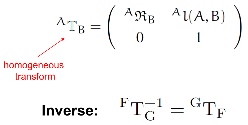
The homogeneous transform#
Unit quaternions are used for the attitude representation within homogeneous transforms.
Spatial notation#
kdFlex uses spatial notation throughout the code base. Spatial
vectors are 6 dimensional quantities with angular and linear components.
The Karana.Math.SpatialVector class is used for spatial vector
instances.
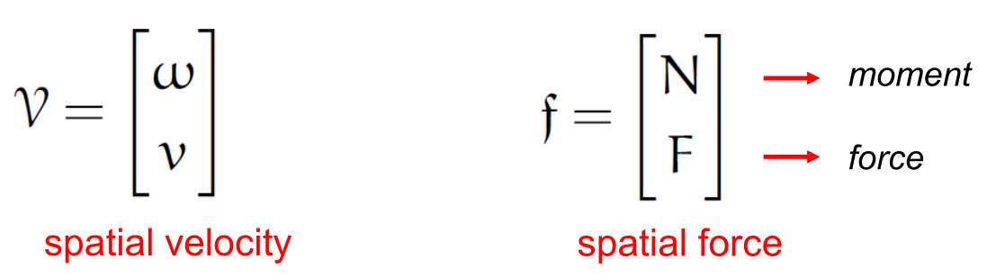
Spatial velocity and spatial force vectors#
By convention, the angular component comes first within a spatial vector,
followed by the the linear component. Thus spatial velocities contain
angular velocities followed by linear velocities, and spatial forces
have the momentum component first, followed by the linear force
component. Spatial notation also extends to spatial inertias which
combine the inertia tensor, with the CM offset vector and the body
mass. The {py:class}`Karana.Math.SpatialInertia} class is available for spatial
inertia instances. For the 3x3 rotational inertia tensors, the
kdFlex convention is to use the negative integral convention for the
off-diagonal terms, so that the matrix is always positive semi-definite.
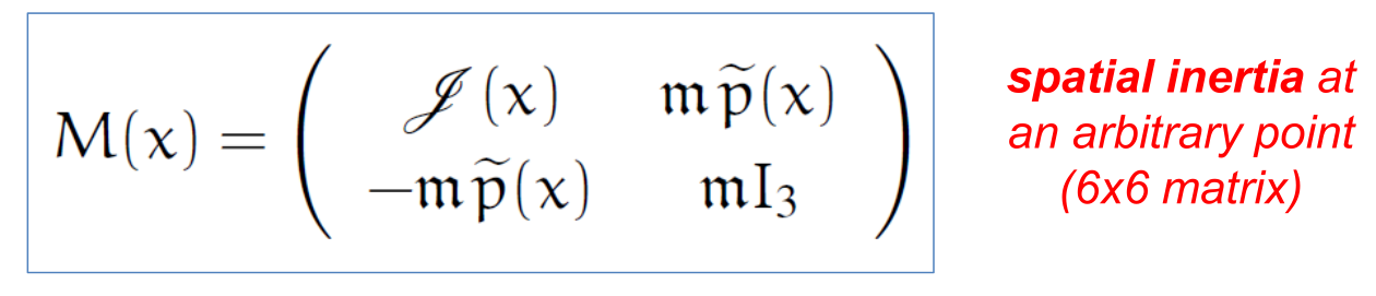
The spatial inertial matrix#
A noteworthy fact is
that homogeneous transform classes have the phi() and
phiStar() methods for carrying out
rigid body transformations of spatial quantities.
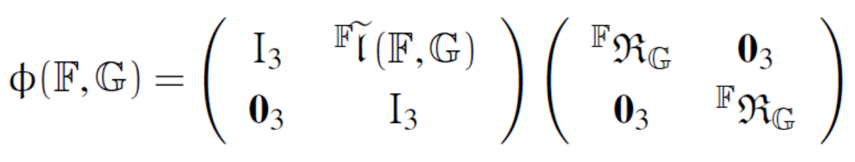
The phi rigid body transformation matrix#
The following summarizes expressions for rigid body transformations of spatial velocities, accelerations, forces, momenta and inertias that can be carried succinctly using these methods.
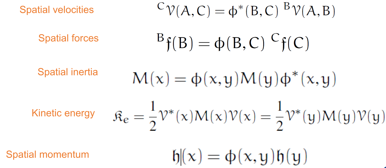
Rigid body transformation examples#
Coordinate Frames#
kdFlex has a general purpose frames layer consisting of a directed
tree of frames. The frame family of classes form a foundational layer
for the multibody classes. Each Karana.Frame.Frame instance represents
a node in a tree of frames managed by a Karana.Frame.FrameContainer
instance. A Karana.Frame.FrameToFrame instance is defined by a pair of
from/to frame instances. The edges in the frame tree are defined by
Karana.Frame.EdgeFrameToFrame instances. Each edge contains
the relative pose across the edge defined by a
homogeneous transformthe relative spatial velocity across the edge defined by a
spatial vectoras observed from and represented in the oframethe relative spatial acceleration across the edge defined by a
spatial vectoras observed from and represented in the oframe
An application is responsible for setting the pose, spatial velocity and
spatial acceleration for each of the edges in the frames tree. The
frames layer provides support for creating frame-to-frame
instances - referred to as chains - from arbitrary oframe/pframe
pairs of frames. Applications can query chain instances for the
relative pose, spatial velocity and spatial acceleration across the
oframe/pframe pair for the chain. The chain instances internally combine
the contributions by the appropriate edges along the connecting path to
compute the overall requested data across the path. The
Karana.Frame.ChainedFrameToFrame chains can be defined using arbitrary
oframe/pframe frame pairs from the frames tree. The
Karana.Frame.OrientedChainedFrameToFrame chains can only be used when
the oframe is an ancestor of the pframe frame.
Creating a frame container#
We start off the creation of a frames layer by creating a
frame container by calling its create()
static method. This creates a frame container with a single
root frame that serves as the anchor for the
rest of the frames in the system.
The frames layer#
Additional frames can be created by calling the frame
create() static method. Each new
frame needs to be attached to a frame in the frames tree. This
can be done by creating a frame-to-frame edge by calling the
Karana.Frame.PrescribedFrameToFrame.create() method. This method takes
a parent and unattached child frame arguments and attaches the child
to the parent in the tree. The first (i.e. the “from”) frame in a
frame-to-frame is referred to as the oframe frame, and the second
(i.e. the “to”) frame is referred to as the pframe frame. That o
comes before p alphabetically mnemonic can be helpful to remember this
naming convention.
While
these are the basic steps to build up the frame tree, other steps, such
as adding bodies and hinges, also add frames to the frame tree. Once the
frames tree has been built, the frame container
ensureHealthy() method
must be called to finalize the tree so that it is ready for use. A
frame can be looked up by name using the frame container’s
lookupFrame()
method. Calling a frame’s
dumpFrameTree() methods displays the frame tree hierarchy
starting with the frame. The
following is example Python code for creating a frame container, adding
frame instances and attaching them.
# create a frame container
fc = FrameContainer.create()
# get the root frame
root_frame = fc.root()
# create a new frame
frmA = Frame.create("frameA", fc)
# attach the new frame to the root frame
f2fA = PrescribedFrameToFrame(root_frame, frmA)
# create a second frame
frmB = Frame.create("frameB", fc)
# attach the B frame to the A frame
f2fB = PrescribedFrameToFrame(frmA, frmB)
# finalize the frame container once the structural changes are done
fc.ensureHealthy()
# display the current frame hierarchy
root_frame.dumpFrameTree()
A frame can be detached from the frame tree by deleting its edge:
# get the edge
e = frm.edge()
# delete the edge
e.discard()
# verify that the edge is gone
assert not frm.edge()
A frame can be reattached by creating a new
Karana.Frame.PrescribedFrameToFrame edge connecting it to another
parent frame. Note that a frame container cannot be made healthy(via
its ensureHealthy()
method) if there are any unattached frames in the
system.
Edge relative data#
The application is only responsible for setting the edge relative
transform spatial velocity and spatial acceleration values. The relative
homogeneous transform for an edge frame-to-frame can be set using its
setRelTransform() method, the
relative spatial velocity using its
setRelSpVel() method, and the
relative spatial acceleration via its
setRelSpAccel() method. The following Python code illustrates how to set the edge data for the
frame creation example above:
# set the edge transform for frmA
f2fA.setRelTransform(HomTran(UnitQuaternion(1, 0, 0, 1), [1,2,3]))
# set the edge relative spatial velocity for frmA
f2fA.setRelSpVel(SpatialVector([3, 4, 5], [1,2,3]))
# set the edge relative spatial acceleration for frmA
f2fA.setRelSpAccel(SpatialVector([4, 5, 1], [.1,0,.6]))
For some frame-to-frame edges, the pose, velocity, acceleration data is fixed
and needs to be set just once (e.g., for rigidly attached frames). More
generally, callbacks can be registered with an frame-to-frame edge to
automatically update the transform and related data. This callback
mechanism is used for auto-updating frame-to-frame edge data for subhinges
after coordinate changes, and changes to ephemeris time for Spice edge
frame-to-frame etc.
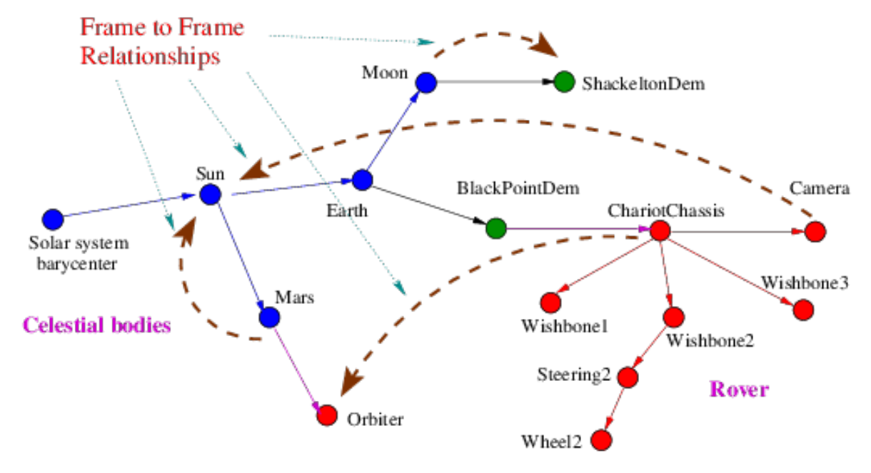
Ephemerides frames#
Karana.Frame.SpiceFrame class is a specialized frame class for frames
associated with celestial and other bodies for ephemerides. For instance, these
frames are associated with celestial bodies in the solar system such as
the Sun, the Earth, the Moon, Mars etc. The
Karana.Frame.SpiceFrameToFrame class is for edges defined by
SpiceFrame oframe/pframe pairs.
The motion of a Spice frame
can queried from ephemeris kernels from the JPL NAIF
toolkit. The
Karana.Frame.SpiceFrame.lookupOrCreate() method can be used to create
such a frame using NAIF body and frame ids. The
Karana.Frame.SpiceFrameToFrame edges are created from pairs of
Spice frames instances. The data for the Karana.Frame.SpiceFrameToFrame edges is
computed for the specified time epoch from the loaded
NAIF kernels. Once created, these Spice frame instances become a part of the
frames tree, and thus can be used seamlessly with any other frame
in the frames layer. Thus for example, querying the direction of the sun, or
the moon from a camera or a sun sensor attached to a terrestrial
platform simply requires the creation of the Spice frame for the relevant
celestial bodies, after which relative transform queries from any other
frame such as the camera can be made directly.
The Spice frames example notebook
contains a
celestarium example to illustrate creating frame container and frame instances
and the use of Spice frames.
Vector time derivatives#
It is important to keep in mind that there are potentially four frames involved when computing time derivatives of vectorial quantities for velocities and accelerations. These have to carefully handled in the presence of rotating frames as is common place for multibody systems. These four frames are:
the first two are the from and to frames that are referred to as the oframe/pframe frame pair.
the next frame is the observing frame, i.e. the frame in which the oframe/pframe relative quantity whose derivative is being taken is represented. The observing frame often is the same as the oframe, but that is not a requirement.
the fourth frame is the representation frame, i.e. the frame in which the derivative quantity (which is itself a vector) is represented. Often this representation frame is the same as the observing frame, but this is again not a requirement.
kdFlex provides the frame-to-frame
relTransform(),
relSpVel(),
and relSpAccel()
methods to return the relative pose, spatial velocity and
spatial acceleration respectively of the oframe/pframe pair frame-to-frame as
observed from and represented in the oframe frame. The kdFlex
frame layer convention is that the oframe is the observing and
representation frame for the quantities returned by these
methods. There are additional methods available to transformation the
data into alternative observing and derivative frame choices (see
the Changing observer and derivative frame section). Another noteworthy observation is
that with rotating frames, there are Coriolis acceleration terms when
working with accelerations, and their specific values depends on the
specific choices of the oframe, pframe, observing and representation
frame.
Arbitrary frame pair relative data#
The frames layer supports on demand computation of relative pose, spatial velocity, and spatial acceleration for any pair of frames in the system. The frame pair may be on arbitrary branches, and the connecting path may involve traversing edges in the opposite direction. Combining the edge relative transform values along the path is taken care of by the frames layer for each of the transform, velocity and acceleration levels.
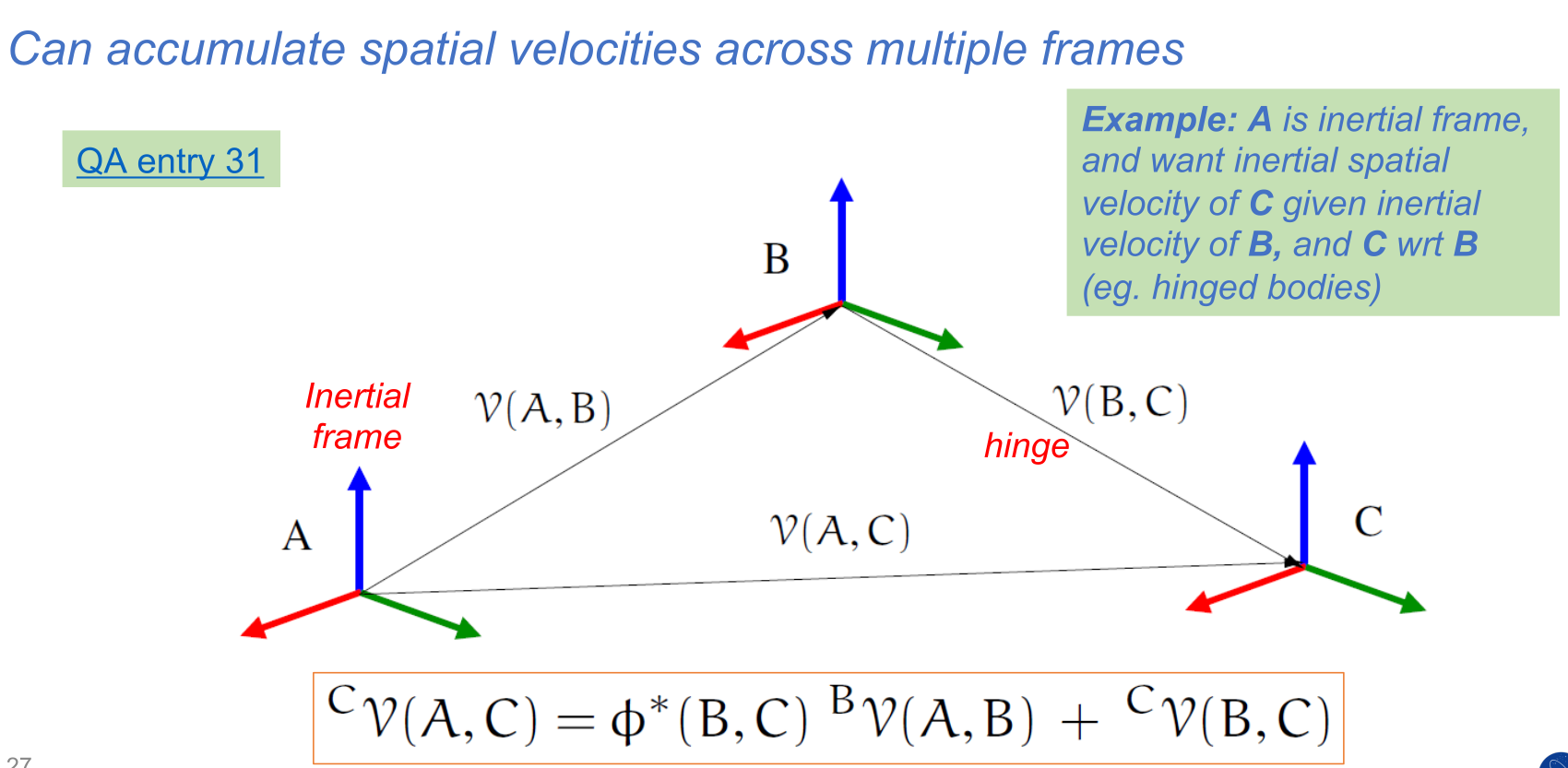
Combining spatial velocities across frames#
This combination process takes into account the transformations needed to combine data from the different oframe, pframe, observing and representation frames encountered along the path.
Calling a frame’s (the from/oframe frame)
frameToFrame() method with a
to/pframe frame argument will return a
Karana.Frame.ChainedFrameToFrame frame-to-frame chain instance with
information about the path connecting its oframe/pframe pair. The
relTransform() method can be called on the
frame-to-frame chain to get the relative transform for the frame pair, the
relSpVel() method for the relative spatial
velocity, and relSpAccel() method for the
relative spatial acceleration of the pframe with respect to the oframe,
with the oframe also serving as the observing and representation
frame. The following code shows how to create a chain and query the
chain’s relative pose etc data for the above
frame creation example:
# get the root/frmB frame to frame chain
f2f = root.frameToFrame(frameB)
# get the relative transform for the chain
T = f2f.relTransform()
# get the relative spatial velocity for the chain
V = f2f.relSpVel()
# get the relative spatial acceleration for the chain
A = f2f.relSpAccel()
# get the oframe and pframe for the chain
of = f2f.oframe()
pf = f2f.pframe()
The user is also free to create chains such as
frameB.frameToFrame(root) where the pframe is an ancestor of the
oframe, or even on a different branch altogether. It is important to
appreciate that this chain’s relative data can well be non-zero, because
even though the root frame is the anchor (and does not move), the
root frame will appear to move when observed from another moving
frame. The frame’s
frameToFrame() method first checks whether the required frame-to-frame
instance already exists or needs to be created, and creates one if
necessary. For applications that have a recurring need for a specific
frame-to-frame, it is a good practice to cache the frame-to-frame instance
locally to avoid the costs from repeated look ups.
Changing observer and derivative frame#
By convention, the frame-to-frame relSpVel()
and relSpAccel() methods compute
quantities relative to the oframe and with the oframe being the
observer frame. Additional methods are available for switching to an
alternative observer frame for vector derivatives. The frame-to-frame
pframeObservedRelSpVel() and
pframeObservedRelSpAccel()
methods return the oframe/pframe relative
spatial velocity and acceleration respectively with the pframe being the
observer frame.
The frame-to-frame
toPframeRelativeSpVel()
and toPframeRelativeSpAccel()
methods go further and are handy methods for transforming hypothetical oframe
relative spatial velocity and acceleration derivatives into pframe relative ones.
The frame-to-frame toOframeObserved()
method can be used to transform arbitrary pframe
observed 3-vector derivative into an oframe observed vector derivative. Thus
assume that we have frame A, a 3-vector \(X\) and its A
observed time derivative Xdot_A. To convert this derivative into
another frame B observed derivative. Xdot_B, run
Xdot_B = B.frameToFrame(A).toOframeObserved(X, Xdot_A)
This method is general can be used for both spatial velocity and acceleration quantities.
Remarks on frames#
Frames are typically created to track locations
of interest in a simulation where bodies are in motion, and subhinges are
articulating. The motion of some of the frames may be driven by the
dynamics of bodies being simulated, while in other cases the motion may
be driven by sources such as ephemeris which defines the motion of
celestial bodies over time. A frame layer that uniformly includes all of
the entities of interest in a simulation allows users to seamlessly make
queries about the relative motion of one frame with respect to another
for frames from diverse and disparate sources. Examples of
specializations of frame classes are bodies and body node
classes. Subhinges are specializations of edge frame-to-frame classes, while
body hinges are specializations of. oriented, chained frame-to-frame classes. It is
thus trivial for example to query the relative transform or velocity of a frame
on one vehicle with respect to another even when there are several moving
frames in between. The frames layer relieves applications from having to
implement custom code for making such frame-to-frame queries. – bespoke implementations
that can often be fragile and error prone.
It is worth remembering that the structure of a frame tree is not unique. The only requirement is that the edge transform and related values be set correctly for the specific frame tree structure.
In practice, there can be hundreds if not thousands of frames in a simulation. Keeping the frame to frame data updated for all frame pair combinations in the frame tree at all times is impractical. Therefore, the frames layer uses an on demand, lazy computation model that computes relative frame pair values on demand. There is also a built in data-caching capability that avoids recomputing frame to frame data that have not changed.
Multibody Layer#
Physical bodies and hinges#
In kdFlex, a multibody system is an instance of the
Karana.Dynamics.Multibody class. The multibody representation consists
of a tree or graph of physical bodies connected by hinges that define
their permissible relative motion. Before turning to the process for
creating multibody instances in the Creating a tree multibody system section, we first describe
the bodies and hinges that populate such multibody models. kdFlex
supports a number of classes for different body types derived from the
Karana.Dynamics.BodyBase class. The different body types are:
the
Karana.Dynamics.PhysicalBodyclass for physical rigid bodiesthe
Karana.Dynamics.PhysicalModalBodyclass for small deformation physical flexible bodies. This class is derived from theKarana.Dynamics.PhysicalBodyclass.the
Karana.Dynamics.CompoundBodycontainer class for a connectedsubtreeofphysical bodyinstances treated as a compound body unit. Compound bodies are notphysical bodiesthemselves.
Note that the physical body class is sub-classed from the
Frame class, and thus physical body instances are
also frames with additional attributes such as mass properties. We
will use the physical body terminology for concepts that only apply to
physical bodies, and just body terminology for ones that even apply to
compound bodies.
Multibody representations#
Within kdFlex, physical body instances are connected
in parent/child relationship via Karana.Dynamics.PhysicalHinge hinge instances.
The physical body members of a multibody system are
organized in a tree structure, with each physical body having at most a single
parent physical body.
A multibody graph system’s closed-chain topology is represented as the
combination of a physical body tree together with an additional set of
cut-joints defined as Karana.Dynamics.LoopConstraintCutJoint
hinge-loop-constraint instances (see Cut-Joint constraints
section). For regular serial and tree topology multibody systems, the
set of constraints is empty. Such graph representations are not
unique. As discussed in Cut-Joint constraints section, physical hinge and
cut-joint loop constraint represent complementary ways of characterizing the
permissible motion between nodes on physical bodies, with a physical hinge providing
an explicit way, and cut-joint loop constraint providing an alternative
implicit way.
While a physical hinge instance can be replaced with an equivalent
cut-joint loop constraint instance, the converse is not always
possible without violating the tree-topology structure requirement for
physical bodies and hinges.
Among the possible graph representations for a multibody system, at one
extreme is a representation where all physical body are independent and
connected to the root via a 6-dof hinge. Thus the
physical body instances do not have children, and the motion constraints
on each physical body is defined via a set of cut-joint loop constraint
instances. We refer to such a multibody representation as a
Fully Augmented (FA) model. FA models are also
referred to as absolute coordinate multibody models in the literature.
At the other end of the spectrum is a multibody graph representation
consisting of a maximal spanning tree of physical bodies connected in a
tree-topology structure via a set of inter-body physical hinge instances,
together with a minimal set of cut-joint loop constraint for cut-joints. We
refer to such a multibody representation as a Tree Augmented (TA)
model. Note that converting all the physical hinge instances in a TA model
representation into cut-joint loop constraint instances turns it into an FA
model representation. Between the span of representations book-ended by
the FA and TA representations lie a whole range of intermediate
representations where only a subset of the physical hinge instances are
converted into cut-joint loop constraint instances.
The number of degrees of freedom (dofs) in a multibody system is defined
by the difference between the number of generalized velocity coordinates
(see Generalized Q, U etc coordinates section) for the multibody system, and the number
of constraints on the system. The number of dofs is invariant for a
multibody
system across the different representations. This does imply
that the number of coordinates and the number of constraints rise and
fall together across different multibody representations since their difference is
fixed.
kdFlex supports both FA and TA multibody representations, and arbitrary
intermediate versions where some of the physical hinges in a TA model are
replaced with cut-joint loop constraint instances. Within this set of multibody
representations, the TA model requires the smallest number of
coordinates to describe the system configuration (and thus also the smallest
number of constraints). The computational cost of the kdFlex SOA based
algorithms typically increases with the number of coordinates,
and thus it is advantageous, and the default, to use TA multibody
representations to the degree possible. There are methods available to
transform among multibody representations. In contrast with
kdFlex, most general-purpose multibody dynamics tools favor the FA
multibody representations because of its simplicity. However, this
simplicity comes with a large computational cost. The SOA methodology
provides tools to manage the increased complexity of TA models, and take
advantage of minimal coordinate representations to develop fast
computational dynamics algorithms. kdFlex uses these SOA-based
algorithms and thus favors TA model representations by default.
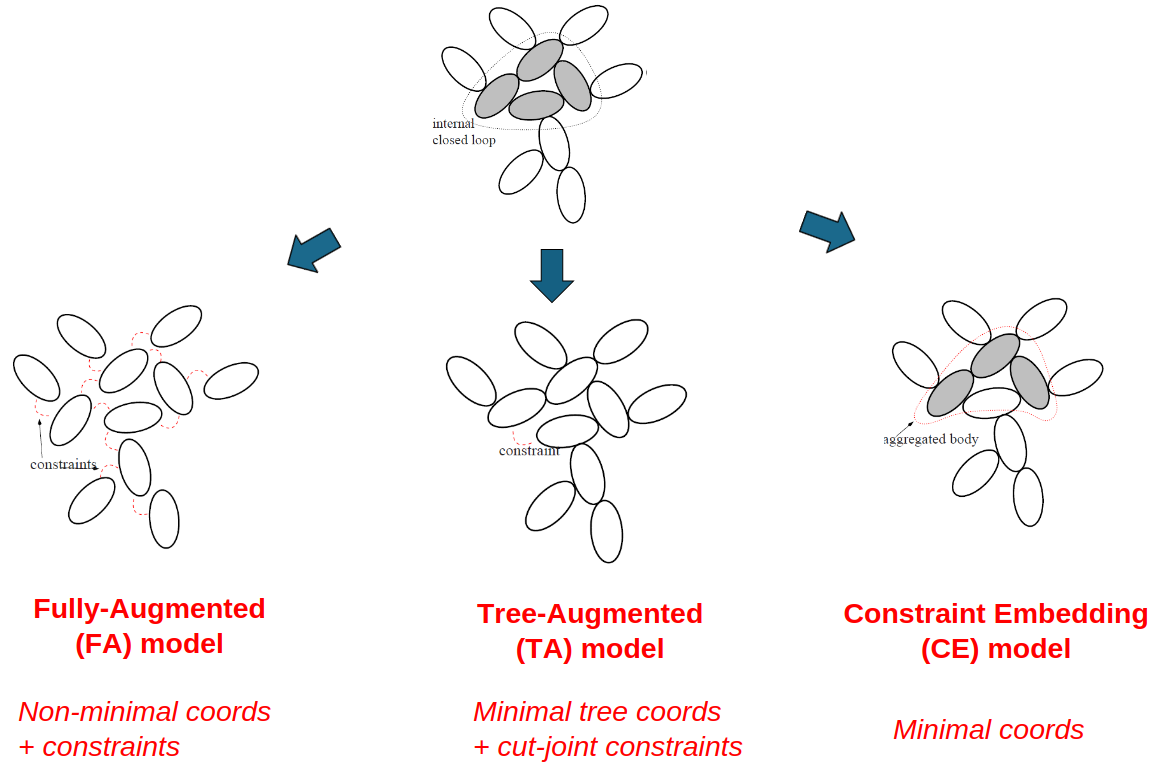
Representation options for a multibody system#
While TA models having a smaller number of coordinates when compared with FA models, TA models are not minimal coordinates when there are loop and coordinate constraints. There is yet another multibody representation, referred to as Constraint Embedding (CE) that is truly minimal. CE models are an advanced topic, that we defer documentation for later.
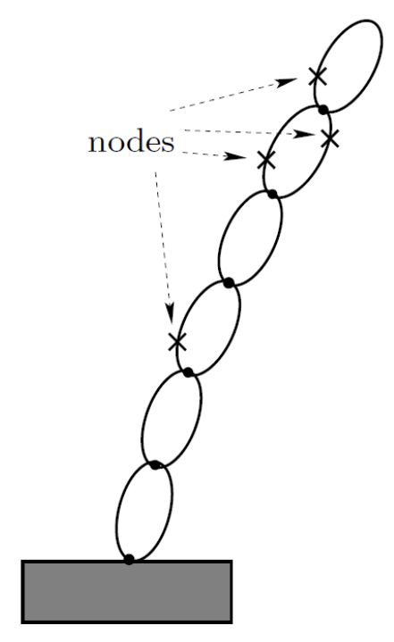
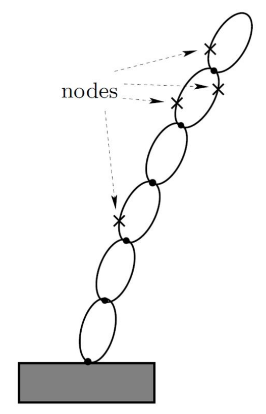
Body nodes#
The Karana.Dynamics.Node class is used for nodes that represent
locations of interest on a physical body. Once a physical body
has been created, node node instances can be created
on the physical body using the Karana.Dynamics.Node.lookupOrCreate() static method. This
class is derived from the Karana.Frame.Frame class and the node instances are
thus also frame instances - albeit attached to a parent physical bodies. One
can think of a node as the special type of a frame
that is directly attached to a physical body.
Node may be used to attach other physical bodies, or represent attachment
points for sensors and actuators attached to the parent physical body. A
node’s setBodyToNodeTransform()
method can be used to set the (undeformed)
location and orientation of a node on its parent physical body. Since
each node is also a frame, it is a simple matter to query a
node’s pose, velocity etc. information relative to any other
frame using the frames layer (see Coordinate Frames
section). Selected nodes can be designated as ones that can apply
spatial forces on the body, and these nodes are referred to as
force nodes. Nodes that serve as attachment points for actuator
devices (e.g., thrusters) that apply forces on a physical body must be
designated as force nodes or else the applied forces will be ignored
during dynamics computations.
While the location of a node on its parent physical body remains
fixed on a rigid physical body instance, the location and orientation of
nodes attached to a physical modal body instance (see Flexible body systems
section for more on flexible bodies) can change as the body deforms.
Body nodes#
Before carrying out any computations, the parameters for all of
the physical bodies and and hinges need to be set. A physical body’s parameters can be set via
its setParams() and other related
methods.
Connecting bodies via hinges#
A physical body is connected to its parent Karana.Dynamics.PhysicalBody via a physical hinge of
Karana.Dynamics.PhysicalHinge type. A physical hinge is a
specialization of the Karana.Frame.OrientedChainedFrameToFrame class.
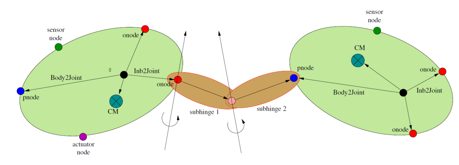
Body pair connected by a hinge#
The hinge creation process automatically creates a pair of node
instances, referred to as an onode of type
Karana.Dynamics.HingeOnode and a pnode of type
Karana.Dynamics.HingePnode. The onode is attached to the parent
physical body and the pnode to the child physical body. These nodes serve as the
oframe/pframe for the physical hinge frame-to-frame chain. The onode and
pnode define the location of the physical hinge on the pair of connected
physical bodies. Every physical body instance has a unique pnode that is the
connection point for its parent physical hinge, and has one or more onode
instances where the physical hinge for each attached child physical body is located.
The location and orientation of the onode on the parent physical body
can be set using the onode’s
setBodyToNodeTransform()
method. The location and orientation of the
pnode on the child physical body can be set using the
setBodyToJointTransform() method
for the child physical body.
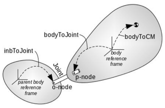
Hinge node locations#
The articulation of the child physical body with respect to the parent physical body is
defined entirely by the relative motion of the hinge’s pnode with respect to the
physical hinge’s onode. The onode and pnode frames for a hinge coincide with the hinge coordinates are zero.
New physical bodies can be attached to existing physical bodies by
creating a physical hinge of a specified type. The
Karana.Dynamics.PhysicalHinge.create() static method creates
physical hinge instances. This method takes a
Karana.Dynamics.HingeType argument to specify the type of
hinge to be created.
The Karana.Dynamics.PhysicalHinge is derived from the
Karana.Dynamics.FramePairHinge class which implements much of the
functionality. The main difference between these classes is that the
latter class simply connects a oframe/pframe frame pair. While the
physical hinge instances are used to connect physical bodies in the multibody
spanning tree. A FramePairHinge
can also be used for defining loop constraint instances (see
Cut-Joint constraints section).
Subhinges#
A physical hinge by itself is a container class for a sequence of zero or
more physical subhinges instances. The
PhysicalSubhinge class is derived
from the Karana.Frame.EdgeFrameToFrame class, and hence represents an
frame-to-frame edge in the frame tree. There are a pre-defined set of
subhinge types selected via the
Karana.Dynamics.SubhingeType available for use. Each
Karana.Dynamics.HingeType enum type corresponds to a
specific pre-defined sequence of subhinge types. The one exception is
the CUSTOM hinge
type which allows the user to specify a custom the sequence of
physical subhinges types.
Generalized Q, U etc coordinates#
Every physical subhinges in the multibody system has a set of generalized
coordinates that parameterize its motion. Additionally, deformable
bodies such as physical modal body have generalized coordinates that parameterize its
deformation. All objects that contribute such generalized coordinates,
including subhinges and physical bodies, are derived from the abstract
Karana.Dynamics.CoordBase class. Each coordinate object instance has an
inherent polarity (i.e. orientation) with its coordinates
parameterizing the relative motion of some frame with respect to
another. Thus the coordinates for a physical subhinges that is part of a
physical hinge parameterize the motion of the outboard child physical body
with respect to the inboard parent physical body (and not the other way
around!).
The kdFlex conventions for generalized coordinates are described below:
The
coordinate objectnU()method returns the number of degrees of freedom (dofs) for thecoordinate objectinstance. ThenQ()method returns the number of configuration coordinates for thecoordinate objectinstance. These values are generally equal, but there are exceptions such as for theSPHERICAL_QUATphysical subhingestype where they are not.each
coordinate objectinstance has a vector of generalized configuration coordinates, denoted Q (of sizenQ()) for the coordinates that parameterize thehomogeneous transformrelative pose across thecoordinate objectinstance. Thecoordinate objectgetQ()andsetQ()methods can be used to get and set theQvalues for thecoordinate objectinstance.each
coordinate objectinstance has a vector of generalized velocity coordinates, denoted U (of sizenU()) that parameterize the relative spatial velocity across thecoordinate objectinstance. Thecoordinate objectgetU()andsetU()methods can be used to get and set theUvalues for thecoordinate objectinstance. In many cases, the U coordinates are the time derivatives of the Q coordinates, but this is not true when using quasi-coordinates (such as forSPHERICALphysical subhingestype), and cases where even their sizes may differ (such as forSPHERICAL_QUATphysical subhingetype)!each
coordinate objectinstance has a vector of generalized acceleration coordinates, denoted Udot (of sizenU()) for the coordinates that parameterize the relative spatial acceleration across thecoordinate objectinstance. Thecoordinate objectgetUdot()andsetUdot()methods can be used to get and set theUdotvalues for thecoordinate objectinstance. TheUdotvalues are the time derivatives of theUvelocity coordinates.
In addition,
each
coordinate objectinstance has a vector of generalized coordinate rates, denoted Qdot (of sizenQ()) for the time derivatives of theQcoordinates. Thecoordinate objectgetQdot()method can be used to get theQdotvalues for thecoordinate objectinstance. TheQdotvalues are auto-computed and thus read-only. TheQdotvalues are often the same asU, except for aphysical subhingesofSPHERICALandSPHERICAL_QUATtypes which make use of angular velocity quasi-velocities for theUvelocity coordinates.a vector of generalized force values, denoted T (of size
nU()) for the forces being applied at thecoordinate objectinstance. Thecoordinate objectgetT()andsetT()methods can be used to get and set theTvalues for acoordinate objectinstance.
Creating a tree multibody system#
The multibody system is the top-level container for all
the physical bodies belonging to the system. Each
multibody instance automatically comes with a virtual
root physical body that serves as the root/anchor for the
actual physical bodies in the system.
kdFlex supports multibody systems with serial-chain, tree and graph
topologies. Unlike serial-chains, tree systems can have branches. The
distinction between tree and graph topology systems is that graphs can
contain loop constraint and coordinate constraint
between physical bodies.
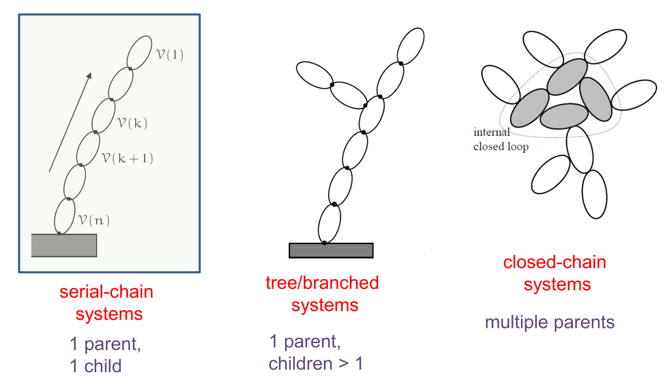
Types of multibody topologies#
A multibody system can be created
procedurally as well from Python DataStruct definitions, YAML, JSON, HDF5 and
URDF model files. Model file exporters to these formats are also
available.
We begin with the steps need to create tree
topology multibody system.
Manual creation#
A multibody system is created by calling the
Karana.Dynamics.Multibody.create() static method. This method takes
as an argument the Newtonian frame which is used as the inertial frame for dynamics
computations. This method creates a multibody instance with a single
virtual root body. This root body serves as an anchor for the remaining
physical bodies that are created subsequently.
New physical bodies can be added to
the multi body system by calling the create() method on the appropriate
physical body class.
Once the physical bodies have been created. The
system. The
Karana.Dynamics.SubTree.displayModel() can be used to display the list of physical bodies and hinges in a multibody system.
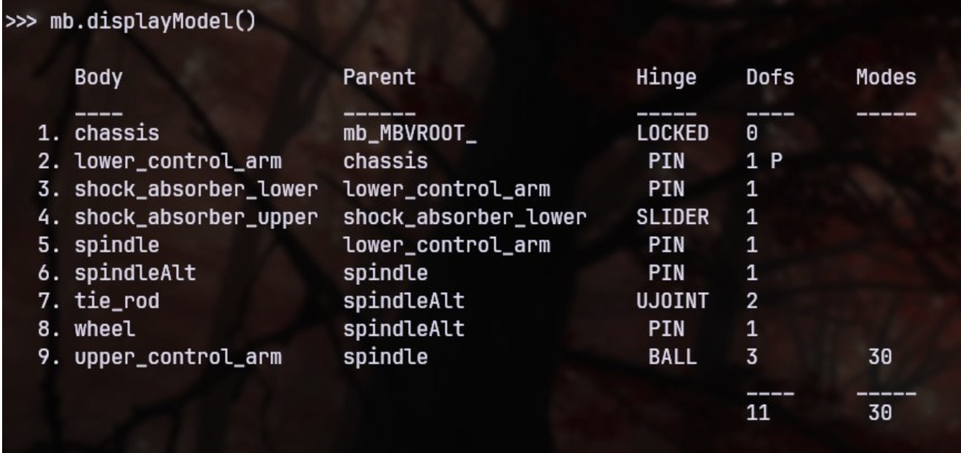
Example output from SubTree.displayModel()#
The Karana.Dynamics.Multibody.dumpTree() method displays the topology of the multibody
system including the loop and coordinate constraints among the physical bodies.
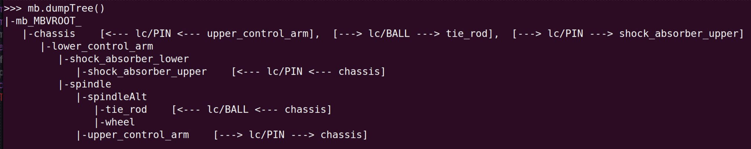
Example output from SubTree.dumpTree()#
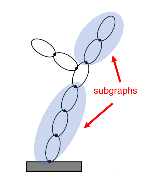
Creating physical bodies and hinges automatically add a number of frames
and edges to the frames tree. You can examine the current state of the
frame tree by calling the dumpFrameTree()
method on the
root frame. An interesting exercise is to identify the segments of the
frame tree contributed by the individual physical bodies, physical subhinges and
physical hinge instances.
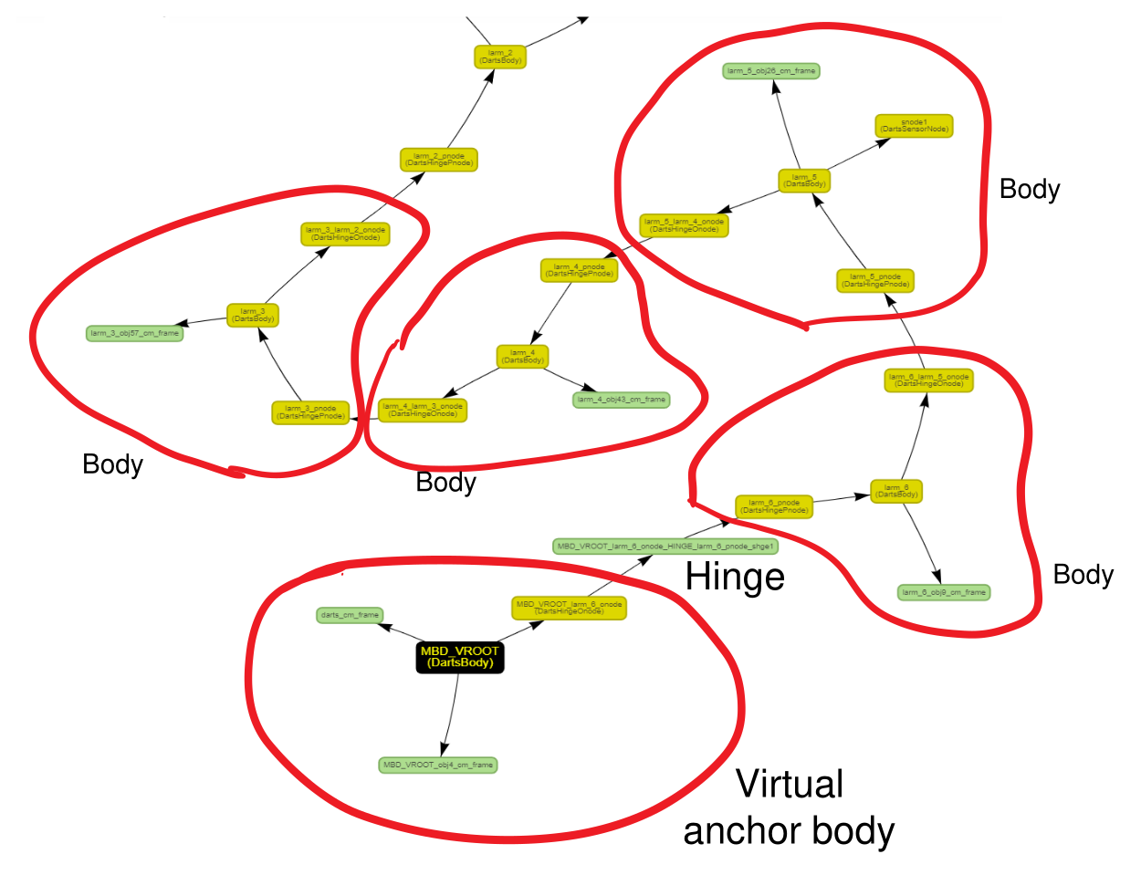
Frames associated with bodies and hinges#
Before carrying out any computations, all of the subhinge and deformation coordinates need to
be initialized (see Subhinges section).
The Karana.Core.allReady() method can be called to
run an audit to verify that there are no unset parameters. It is
a good practice to call this method after multibody system creation and
initialization.
The 2 link pendulum (basic) example script
illustrates the the manual process for creating a multibody system.
The CoordData container#
In a multibody system is created, the collection of physical subhinge and physical modal bodies
together define the system dofs. The
Karana.Dynamics.CoordData container class can be used to manage collections of such
coordinate object instances. For this purpose, the multibody
model has
a
coordinates datainstance for all of thephysical subhingesinstances, and it can be accessed via themultibody’ssubhingeCoordData()methoda
coordinates datainstance for all the deformation coordinates for thephysical modal bodies, and it can be accessed via themultibody’sbodyCoordData()methoda
coordinates datainstance for all thecut-joint loop constraintcoordinates, and it can be accessed via themultibody’scutjointCoordData()method
The coordinates data class provides methods such as nQ(), getQ(), setQ()that parallel the methods
for individual subhinges, except that they work for lists of
coordinate object instances. Thus the Q vector is the combined vector of
the values from each of the subhinges. (See the Generalized Q, U etc coordinates section
for more information on Q, U etc coordinates.) The
dumpState() is handy for
displaying the coordinates data for a coordinates data’s elements.
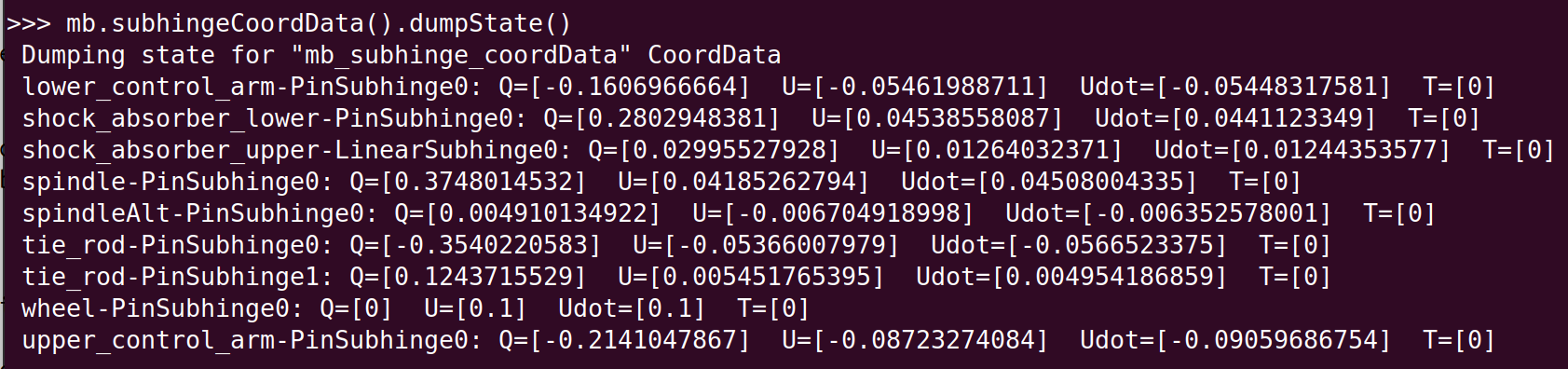
Example output from CoordData.dumpState()#
When getting or setting the Q etc coordinates for a coordinate object,
it is possible to do this directly via the coordinate object instance. This
can be also be done indirectly via a coordinates data instance that
contains the coordinate object instance. To do the so, you will need to find
the correct slot (via the coordinates data’s coordOffsets()
method) for the coordinate object in the overall coordinate vector and get/set these
values. While technically doable. the direct approach is more convenient
to work with for individual coordinate object instances.
Procedural creation#
the previous section described the process for manually creating physical bodies
one at a time. This process provides complete control over creating the right
body types, hinge types and setting up the parent/child body relationships.
Convenience methods are however available to add serial-chain and
tree topology systems of physical bodies to a multibody system. in bulk. The
Karana.Dynamics.PhysicalBody.addSerialChain() and
Karana.Dynamics.PhysicalBody.addTree() methods will create a
serial and tree systems respectively of uniform physical bodies. These methods
are especially useful for automating the creation of large multibody
systems for testing and benchmarking performance. These methods can be
called multiple times to build up the physical bodies in the multibody
system. While these methods create uniform physical bodies, it is
possible to alter the properties of physical bodies individually as desired.
The n link pendulum (procedural)
example illustrates the procedural creation of a multibody system.
Importing model data files#
There is also support for creating multibody systems from model data
files. The following model formats are currently supported:
URDF format model files widely used by the robotics community
The JPL DARTS dynamics simulation tool Python model format files
The SOADyn_types.MultibodyDS DataStruct generated
yaml,json,HDF5andPythonformat model files.
There is also support for exporting model files into the URDF and SOADyn_types.MultibodyDS DataStruct compatible formats.
The WAM arm and M2020 rover
example notebooks illustrate process for creating a multibody system from model files.
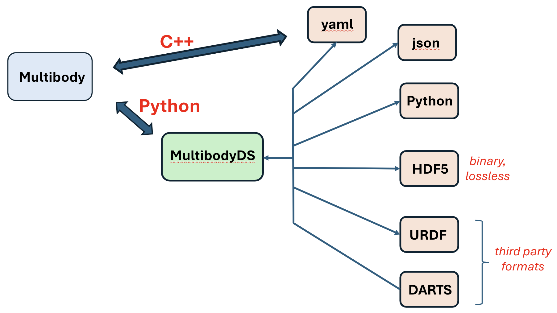
Supported multiple multibody model file import/export formats#
Flexible body systems#
In addition to multibody dynamics with rigid physical bodies, kdFlex also
supports dynamics with flexible bodies, where the rigid/flex dynamics
coupling is rigorously handled using the low-cost SOA dynamics
algorithms. The FEMBridge toolkit provides interfaces for processing
finite-element-model (FEM) data from structure analysis tools such as
NASTRAN to generate assumed modes models for component deformable
bodies. Modeling of flexible multibody system dynamics accurately and
fast, allows kdFlex to support the needs for loads and structures
analysis, as well as for control-system design and analysis. It can
provide accurate and fast performance needed for closed-loop time-domain
simulation testbeds as well as generation of linearized state-space
models for frequency-domain analysis.
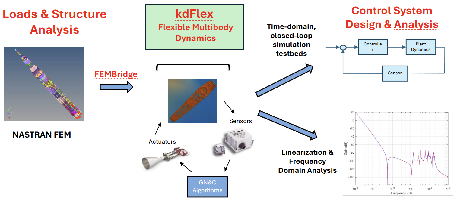
Multibody dynamics bridge between structures and controls discipline analysis needs#
The flexible bodies are assumed to undergo small deformation. The flexibility data for such bodies is typically developed using FEA tools such as NASTRAN. Since these FEA models are typically high-dimensional, an assumed modes approach, together with component mode synthesis (CMS) is typically used to develop reduced order models for the flexible bodies.
Multibody systems with deformable bodies#
Creating flexible bodies#
A flexible body can be created in kdFlex using the
Karana.Dynamics.PhysicalModalBody.create() method. The number of
modes is an argument for this create() method. The
nU() method can be used to query
the number of modes for a body. Note that the returned value from this method is zero for rigid
physical bodies.
The parameters - over and beyond those for a rigid body - for a physical modal body, consist of
a modal stiffness vector defined by the modal frequencies. This can be set using its
setStiffnessVector()method.a modal damping vector. This can be set using its
setDampingVector()method.nodal vectors of size
6xnU()for everynodeon thephysical modal body(includingpnodeandonodeinstances). These nodal matrices are defined from the mode shapes generated by the external model reduction process. Eachnodeon aphysical modal bodyhas a non-nullKarana.Dynamics.ModalNodeDeformationProviderinstance which can be accessed via thedeformationProvider()method. The ItssetNodalMatrix()method can be used to set the nodal matrix for thenode.
Deformation coordinates#
Physical bodies are coordinate object objects. The generalized coordinates
associated with a physical modal body are its deformation coordinates. The
number of deformation coordinates can be queried using the body’s
nU() method. Deformable bodies have nU() size Q,
U, Udot coordinates as described in the Generalized Q, U etc coordinates section
for coordinate object objects. The
getQ() etc
methods can be used to get and set these coordinates. The multibody
instance has a dedicated coordinates data instance with the deformation
coordinates for physical modal bodies that can be accessed via the
CoordData() method.
Virtually all the kdFlex algorithms, including kinematics,
Jacobians, loop constraints, dynamics etc, work for rigid as well as
flexible bodies. This allows kdFlex to support arbitrary graph
topology systems with arbitrary mix of rigid and flexible bodies. This
general capability thus provides accurate and fast rigid/flex multibody
dynamics support capitalizing on the fast SOA methods.
Multibody configuration changes#
kdFlex supports the run-time changes to the multibody system topology. The
Creating a tree multibody system section described the steps for creating a new body. These
steps can be done at any time to add a new body. Removing a body is done by
simply calling the discard() method on the body after all dependencies
have been removed as discussed in the Creating and discarding objects section.
kdFlex also supports changing multibody topologies from detaching
and reattaching bodies as follows.
Calling the
detach()method for aphysical bodywill detach it from its current parentphysical bodyand will delete their connectingphysical hinge. It will also create a newphysical hingeof the specified type to attach the body to themultibodyvirtual root body via aFULL6DOFhinge. The newphysical hingescoordinates are initialized so as to preserve the inertial pose, spatial velocity and spatial acceleration of the body across the detachment action.The
reattach()method can also be called with a new parentphysical bodyargument. This will carry out steps similar to thedetach()method, except that the newphysical hingeof the specified type is created and used to connect the body to the new parentphysical body. If the hinge type isFULL6DOF, then the new hinge coordinates are initialized to preserve the inertial pose, spatial velocity and spatial acceleration of the body across the reattachment.
The inertial pose, velocity and acceleration of the the body are
automatically preserved only for a 6-dof physical hinge type. This is based
on the fact that it is the only hinge type capable of ensuring
continuity in the inertial pose, velocity and accelerations of the body
across the reattachment. Furthermore, using 6-dof hinges is simpler
since they do not require the additional data such as the location of
the new onode and pnode, and additional axes etc parameters.
What about reattaching with a physical hinge type different than a 6 dof
hinge as may be needed in practice while preserving inertial pose,
velocity and accelerations of the physical body. The following describes
the general process for changing the physical hinge type.
to avoid the non-physical discontinuities in
physical bodyinertial pose and velocities, it is necessary that the relative pose, spatial velocities and accelerations of the body with respect to its new parent be achievable by the new desired hinge type. In practice, this may require a transition period (e.g., nulling out relative velocities during a docking scenario) to meet this requirement.once the admissible relative pose etc conditions have been met for the new
physical hingetype, record the new parent relative pose etc quantities - they will be needed later to initialize the newphysical hinge’s coordinates. Thediscard()method on the existingphysical hingecan be called to remove it, followed by a call toKarana.Dynamics.PhysicalHinge.create()method to create the newphysical hingeof the right type between the new parent and thephysical body.now set the
onode,pnodelocations and the axes etc parameters as needed for the newphysical hinge. These steps are similar to the ones needed when attaching a newly createdphysical bodyvia aphysical hingeas described in the Manual creation section.the final step is to set the
physical hingecoordinates to preserve the body’s original inertial pose etc. This can be done by calling thephysical hingefitQ()method to find the bestQcoordinates for the desired relative transform. This method will return the residual transform error, which should be zero if the desired relative transform is compatible with the new hinge type. Similarly calls to thefitU()method should be made to initialize theUcoordinates for thephysical hinge, andfitUdot()method to initialize theUdotcoordinates for thephysical hinge.
After making such changes, it is important to make the
multibody system current to
update it for the new configuration.
Due to the structure-based nature of the SOA algorithms, very little beyond these changes to the topology is needed for all the kdFlex algorithms to continue working. Most of the algorithms are structure-based and will simply start following the new system topology! There is no other bookkeeping updates needed for the changes to connectivity that may otherwise be required in conventional approaches. The cost of making these changes is very modest, and so easy to accommodate in complex scenarios.
Bilateral closure constraints#
Bilateral constraints can be imposed to limit the admissible motions of
physical bodies. Such constraints are can be imposed directly on the body
subhinge coordinates or on the relative spatial velocity of physical
body nodes. The former are referred to as coordinate constraints (see
Coordinate constraints section), while the latter as loop
constraints.
The presence of constraints implies that the system has non-minimal coordinates. By default this requires constraint kinematics solvers (see Constraint kinematics section) to compute system states that satisfy the loop motion constraints. Any meaningful use of such closed-chain topology systems requires that the system states be such that the loop motion constraints are satisfied! Also, different solution techniques for the system dynamics are required since the algebraic motion constraints make the system dynamics model into a DAE system. SOA’s constraint embedding technique can be used to get back to an ODE formulation, but that is an advanced topic for later.
Cut-Joint constraints#
Hinges provide an explicit way to characterize the permissible
constrained between a pair of physical bodies. An alternative,
kinematically equivalent - albeit implicit - way, is to define the
motion constraints via cut-joint constraints. The cut-joint loop constraint
class defines bilateral loop constraints between physical bodies. This
class takes advantage of the duality between hinges and constraints - in
that admissible motions can be defined explicitly using a physical hinge, or
implicitly via a cut-joint loop constraint.
A cut-joint loop constraint can be created using the
Karana.Dynamics.LoopConstraintCutJoint.create() method. A cut-joint loop constraint
is typically created between a a pair of constraint node nodes of type
Karana.Dynamics.ConstraintNode instances attached to a pair of
physical bodies to constrain their relative motion. The same method also
can be used to create a motion constraint between a physical body and the
environment. The method takes a frame-to-frame instance as argument to specify
the frame pair being constrained. At least one of the frames is
required to be a constraint node. The method also takes a
HingeType argument to specify
the allowed motion across the cut-joint loop constraint. A
FramePairHinge instance of the
specified hinge type is used internally to restrict the admissible
motion for the cut-joint loop constraint. This process allows us to use
rigidly locked constraints, as well as more general cases where the
motion is only partially constrained. When the motion is only partially
constrained, there are additional generalized coordinates for the hinge
associated with the cut-joint constraint.
The cut-joint loop constraint
poseError() etc
methods can be used to compute the constraint error for individual
constraints.
Cut-joint constraints are required for multibody systems with graph
topologies, i.e. ones with topological loops. A set of cut-joint loop constraints for the cut-joints, together with the physical bodies subtree, are used by kdFlex to define
general graph topology multibody systems.
While another conceivable option to convert a graph into a tree might be to split bodies rather than hinge, we do not adopt this option. There is no reasonable way to split the mass and modal properties of flexible bodies across the fracture parts. The extreme option of splitting a body while apportioning all the body properties to one part, and making the other part a dummy mass-less rigid body is also problematic since some algorithms cannot accept mass-less leaf bodies.
modes bases. For rigid bodies, we can simply spit about the body frame and assign half mass properties to each half.
The Slider-crank with loop constraints example
illustrates the creation of cut-joint loop constraints for a graph topology
multibody system.
Convel loop-constraints#
Unlike cut-joint loop constraints, convel loop constraints instances do not have a
physical hinges. A convel loop constraint requires projections of the relative
spatial velocity of a pair of physical bodies along an axis to track each
other. Furthermore, a convel loop constraint does not apply at the
relative pose level, and only applies at at the velocity and
acceleration levels. A convel loop constraint is an instance of the
Karana.Dynamics.LoopConstraintConVel class. Since a
convel loop constraint does not have a physical hinge, there are no coordinates
associated with them either. A convel loop constraint can be either on the
relative angular or linear velocities, and the component axis can be set
via its setUnitAxis() method.
Both the cut-joint loop constraint and convel loop constraint classes derive
from the LoopConstraintBase
class. This class’s hasHinge() method can
be used to distinguish between these two loop constraint types.
Coordinate constraints#
While cut-joint loop constraint and convel loop constraint instances restrict
the admissible spatial velocity across constraint node and frame
instances, a coordinate constraint directly imposes algebraic constraints
between generalized coordinates to restrict their motion. Examples of coordinate
constraints are physical bodies coupled via gears, with their respective
generalized coordinates values being subject to a fixed scalar ratios.
The Karana.Dynamics.CoordinateConstraint.create() method can be used to create a coordinate constraint instance to impose a
scale ratio between the Q coordinates of a pair of physical subhinges (with the
same number of dofs). The scale ratio can be set via the
setScaleRatio() method. This
coordinate constraint can be used for a pair of rotational physical subhinge (e.g., for gears)
or the combination of rotational and translational physical subhinge, such as for
rack and pinion mechanisms.
Sub-Trees#
While most applications will carry out computations on the full
multibody system, it is possible to restrict computations to a
connected set of physical bodies in the multibody system. For
instance, for simulations with multiple vehicles, the user may at times
want to limit some of the kinematics, statics or dynamics computations
to individual vehicles. A similar story applies to multi-limbed robotic
systems where some tasks may involve just a sub-set of the limbs. An
additional pertinent example would be mobile manipulator systems where
the computations can be narrowed down to just the manipulator for
scenarios where the mobility degrees of freedom are not active. The
Karana.Dynamics.SubTree class is a container class for a sub-tree of
physical bodies for this purpose. The physical bodies of in this container
must for a topological tree, and thus the sub-tree must have a single
virtual root body that is the ancestor of all the physical bodies in the
sub-tree.
The Karana.Dynamics.SubGraph is a derived class
that additionally can have a list of
cut-joint loop constraint and
coordinate constraint instances defining the loop and
coordinate constraints between its physical bodies. The Karana.Dynamics.Multibody class itself is
derived from the SubGraph class. All additional
subtree and subgraph instances are children of the parent multibody
system, and contain subsets of the physical bodies in the multibody system.
The Computational Algorithms section describes a number of
available system-level algorithms for kinematics, statics and dynamics
computations that work on subtree and subgraph instances. These
algorithms ignore the physical bodies, physical hinge and frames external
to them when carrying out their computations. This generally means that
the external bodies and frames are treated as kinematically frozen, and
the mass properties of inboard and outboard bodies are ignored. Since a
multibody is also a subtree and a subgraph, passing in the
multibody allows the use of the same algorithm methods for the full
system as well.
A new subtree is created from an existing
subtree instance by calling the
Karana.Dynamics.SubTree.create() method. This method takes the
new_root, use_branches and stop_at arguments to tailor the physical bodies
parent sub-tree to be included in the new sub-tree. The following
describes the role of these options in more detail:
To create a
subtreethat includes all the descendants of a specific body, specify the body as thenew_rootargument and empty lists for theuse_branchesandstop_atarguments. Note that the the specified body will be the virtual root of the newsubtree, and hence technically not belong to it. To actually include this body, specify the body’s parent body (or another strict ancestor) as thenew_rootargument. You can also specify theparent_subgraph.virtualRoot()as the argument value if the body happens to be a base body for the parentsubtree.If the
use_branchesargument is an empty list, then all branches starting from thenew_rootare included in the newsubtree. If a non-empty list of bodies specified as theuse_branchesargument, the included bodies are limited to only those on branches containing one of these bodies. Theuse_branchesargument can thus be used to exclude unneeded branches in the parentsubtree. If thenew_rootargument is null, then the new-subtree uses the common ancestor body for theuse_branchesbody as the root of the newsubtree. Thus at least one of thenew_rootoruse_branchesarguments is required to be non-null.When the
stop_atargument is an empty list, all bodies in the branches specified by thenew_rootanduse_branchesarguments are included in the newsubtree. When thestop_atlist is non-empty, bodies that are descendants of bodies in thestop_atlist are excluded from the newsubtree. Bodies in thestop_atlist are required to be strict descendants of the new root body - since otherwise this would lead to an emptysubtree.A common situation is the need to create a
subtreeconsisting of the minimal spanning tree of a set of bodies. Such asubtreecan be created by specifying a nullnew_rootargument, and the same list of bodies as theuse_branchesand thestop_atargument.
Arbitrary levels of nesting are allowed for subtrees, and a subtree
can have an arbitrary number of children subtrees.
A subtree’s virtualRoot() method can be used to get its root body. Since the set
of bodies can vary across subtree instances, so can the children
bodies for a body. The
childrenBodies()
method can be used to query the children bodies for a
body in a subtree. Since multibody instance is also a subtree,
calling childrenBodies()
method on the multibody returns the full list of
children physical bodies for physical body.
One handy feature of any subtree instance is that it automatically
has a dedicated frame (accessed via its
cmFrame() method) to track the
center of mass location of the bodies in the sub-tree. As a consequence,
a multibody system also has such a CM tracking frame. Since this is a
frame instance, it is a part of the frames tree, and thus the
location of a subtree’s CM location can easily be queried with respect
to any other frame in the system.
Sub-Graphs with Constraints#
The Karana.Dynamics.SubGraph class is derived from the
Karana.Dynamics.SubTree class, and adds support for
bilateral loop constraint and coordinate constraint
constraints (see Bilateral closure constraints section) among the subgraph component physical bodies. A subgraph
instance can be created using the
Karana.Dynamics.SubGraph.create() method. In addition to the
arguments for the Karana.Dynamics.SubTree.create() method - for
selecting the bodies to include - the subgraph, this create()
method takes lists of loop constraint and coordinate constraint instances from the parent subgraph to include in the new
one. For convenience, a new subgraph instance automatically
inherits and enables all the constraints from the parent subgraph that are legal for the subset of bodies in the new subgraph. Such inheritance can be disabled by setting the
inherit_constraints argument for the create method to false.
SubGraph illustration#
All constraint instances can be enabled and disabled for a
subgraph at run-time by calling its
enableConstraint() and
disableConstraint()
methods respectively. Only the enabled constraints
are taken into account in computations involving the subgraph. This
provides a convenient way to handle scenarios where constraints are
changing at run-time such as during robot manipulation and mobility
activities.
The Karana.Dynamics.Multibody class is a specialization
of the Karana.Dynamics.SubGraph class. Multiple subtree and subgraph
classes can be created with different combinations of physical bodies and
constraints for a multibody system.
Several of the computational algorithms in kdFlex act on
subtree and subgraph instances. So
while these algorithms can be invoked on the multibody instance, they
can also be called on subtrees and subgraphs. This allows an application to
restrict the execution of these algorithms to a narrower set of the physical bodies
in the multibody system (e.g., to just the manipulator arm on a mobile
platform, or to a single vehicle in a multibody system with multiple
vehicles).
Jacobians#
In the domain of robotics, Jacobian matrices play an important role. In the most basic case, Jacobians relate joint velocities to spatial velocities of a robot end-effector. Jacobians are configuration dependent and need to be computed on the fly in the context of robot motion control since the coordination of multiple limbs is required. In the broader context of multi-limb robots, there are multiple end-effectors. The concept of a Jacobian extends naturally to such multiple end-effectors.
Again, in the context of robotics, Jacobians are needed for inverse kinematics (IK) solvers. The IK problem is one of finding a set of hinge coordinates that will position one or more end-effectors in a desired pose. This typically requires numerical solvers that often utilize these Jacobians within an iterative numerical search process.
kdFlex includes support for the efficient computation of general purpose Jacobians, as well as broader constraint kinematics solver capabilities. For this, kdFlex first generalizes the notion of a Jacobian. Conventionally Jacobians are used to characterize end-effector poses and velocities with respect to the ground or the inertial frame. A more general setting is where the Jacobian is defined for a pair of frames, where both frames may be in motion. In this more general setting, the Jacobian characterized the relative motion between these pair of frames as a function of the joint coordinates. This approach subsumes the conventional case where the Jacobian is with respect to the inertial ground frame. This broader framing allows the use of the Jacobians for the more general constraint kinematics (CK) problem of solving for the system state that satisfies a set of loop constraints.
Jacobians can be relative as well for multiple nodes#
The Karana.Dynamics.FrameToFrameJacobianGenerator.create() method can be
used to create a Jacobian generator for a frame pair defined
by a single frame-to-frame instance for coordinates defined by a coordinates data instance. This object’s jacobian() method computes the
relative Jacobian for the frame pair. The object does the caches
bookkeeping information for reuse across multiple Jacobian calls. By
default, analytical techniques are used to compute the Jacobians. The
Karana.Dynamics.MultiJacobianGenerator class is a more
general version of the generator that can compute the Jacobian for a
list of frame-to-frame instances. Methods such as the
Karana.Dynamics.SubTree.subhingeCoordData() can be used for
the The coordinates data arguments when seeking Jacobians for all the
subhinge coordinates in a subtree.
Constraint kinematics#
The Karana.Dynamics.ConstraintKinematicsSolver class is a general
purpose constraint kinematics solver for solving a subgraph’s
coordinates that satisfy its motion constraints. The simplest way to
create an instance of the solver is by calling the subgraph’s
cks() method. This solver will be
setup to solve for the subgraph state satisfying its enabled
constraints. The solver’s
solveQ()
etc methods can be invoked to solve for the coordinates satisfying the
constraints. The returned value is the residual error.
The frozen coordinates are left unchanged during the solution process.
A feature of the kdFlex constraint kinematics solver is that it allows
for the freezing of a subset of the subgraph coordinates using the
freezeCoord()
method. Such freezing can be useful for subgraphs
with redundant coordinates, where the overall strategy may be to use
additional policies to manage a subset of the coordinates, and shield
them from change during the solution processes.
The Slider-crank with loop constraints example illustrates the creation of and use of constraint kinematics solvers.
Inverse kinematics#
In its simplest form, the inverse kinematics (IK) problem is one of solving for joint coordinates required to achieve a desired pose for a frame such as the end-effector. We recast the IK problem into a constraint kinematics problem by creating a loop constraint whose satisfaction would meet the IK requirements. We can then proceed to use the constraint kinematics solver’s solve methods to obtain the IK solutions. This approach is quite general, and allows us to solve IK problems involving relative pose requirements across moving frames, having multiple such requirements, and accommodate cases where the relative pose requirements are partial - such as position only, or orientation only.
Consider for instance a multi-limbed robot, where the scenario calls for using one limb end-effector to anchor the robot by holding on to a handle, while planting one end-effector on the floor, and using two other limbs to grasp and move a task object from one position to another. Motion planning for this scenario requires solving the inverse kinematics for the robot across the whole motion trajectory. The following steps can be used to carry out the coordinated motion for the robot using kdFlex:
Create a
cut-joint loop constraintconstraint of hinge of typeKarana.Dynamics.HingeType.LOCKEDbetween the planted end-effector and the ground, and add and enable it in thesubgraph.Create a
cut-joint loop constraintof typeKarana.Dynamics.HingeType.LOCKEDconstraint of hinge between the end-effector holding the handle, and the handle, and add and enable it in thesubgraph.Create a pair of
cut-joint loop constraintconstraints of hinge typeKarana.Dynamics.HingeType.LOCKEDbetween each of the end-effectors holding the task object and the point of attachment on the task object, and add and enable it in thesubgraph.Enable the IK constraints in the
multibodyinstance by calling theenableConstraint()method for each of them.Call the
multibodycks()method to get theconstraint kinematics solverinstance for themultibody.Select the subset of independent coordinates to use to parameterize the motion. These can be external coordinates, such as the desired position of the task object, along with redundant hinge coordinates within the
multibody. Use thecksfreezeCoord()method to freeze the coordinates that we do not want the IK solver to change (i.e. the independent coordinates).Now set the independent coordinates to their (frozen) coordinate values. Then call the
constraint kinematics solversolveQ(),solveU()andsolveUdot()methods as needed to solve for theQ,UandUdotcoordinates satisfying the constraints. The return value from these methods is the residual error - which should be zero if the IK solution was successful. The solution coordinates will be stored at within eachphysical subhinges, and the values can be queried individually, or for the fullmultibodyby calling it’sgetQ()etc methods. An important reminder is to always do theQ,UandUdotsolutions in order, since each solution depends on the previous one. If solving for IK coordinates across a path, this step can be repeated over over with new values for the independent coordinates to get the matching set of IK solutions.Once done with the IK solutions, disable the IK constraints from the
multibodyby calling thedisableConstraint()method for each of them. Also, unfreeze the independent coordinates by calling the thecksunfreezeCoord()method.
If the IK solutions are required multiple times during the simulation
scenario, an option is to create a dedicated subgraph instance
for IK solutions with all the bodies in the system. The user simply
needs to use the subgraph instead of multibody in the
steps above for the IK solution. The advantage of this approach is that,
the enabling of constraints, and freezing of coordinates just needs to
be done once - or as changes happen, without the need to undo them after
use.
Dynamics Computations#
While the classes described above can be used to define the multibody
system model, the Karana.Dynamics.Algorithms class contains several
static methods for system level computational algorithms. The algorithms
described here are are atomic, work-horse methods that are available for
use by higher level layers in an application. These methods carry out
computations for a specific state of the system, and use the Q and U
generalized coordinate values set in the multibody
system when a method is called. Thus the kinetic energy method computes
the kinetic energy at the state set in the multibody instance. Before
getting to the algorithms themselves, we first pause to introduce the
notion of prescribed motion that is important for the forward
dynamics related algorithms.
Hybrid Forward Dynamics and Prescribed Motion#
The conventional inverse dynamics problem is one of using the
equations of motion to compute the T generalized forces for an input
set of Udot generalized accelerations. The conventional forward
dynamics problem is the converse, and involves using the equations of
motion to compute the Udot generalized accelerations for an input set
of Udot generalized forces. However, there are times when the
situation is mixed, and the inputs are a combination of T generalized
forces at some subhinges and the Udot generalized accelerations at the
remaining ones, and we need to compute the complimentary unknown
generalized forces and accelerations. For this situation, the subhinges
with input Udot generalized accelerations are referred to as ones
undergoing prescribed motion since their motion problem is
pre-determined. The physical subhinges
setPrescribed()
method can be used to set and unset its prescribed motion property. By
default, physical subhinge are non-prescribed.
kdFlex includes support for the mixed situation with a hybrid forward
dynamics algorithm. This algorithms will use the T generalized force
values of non-prescribed physical subhinge as input and the Udot
generalized acceleration values for prescribed ones. The hybrid
algorithm will compute the unknown Udot values for the non-prescribed
physical subhinge, and the T values for the prescribed ones. When none of
the physical subhinge are prescribed, we fall back to the conventional
forward dynamics problem. On the other hand, when all physical subhinge are
prescribed, the resulting computations are those for the inverse
dynamics problem. The kdFlex forward dynamics algorithm is in fact the
hybrid forward dynamics algorithm so it can handle the the conventional
inverse and forward dynamics cases, as well as the hybrid in-between
cases. For the pure inverse dynamics case, there are however faster
alternative Newton-Euler methods available for carrying out the
computations.
A noteworthy fact is that the prescribed property for any physical subhinges can
be changed at any time during a simulation, and the hybrid algorithm
will seamlessly adapt to the changes without any overhead.
The equal and opposite spatial force between physical bodies at the
physical hinges is often of interest. This quantity corresponds to Lagrange
multipliers that are solved for in absolute coordinate dynamics
formulations such as for the Fully-Augmented (FA) models. The kdFlex
ATBI forward dynamics algorithm does not need or compute these
quantities by default. However, these inter-body forces are easily
computed from the ATBI algorithm intermediate quantities, and this
technique is used by the onode
getInterBodyForceTreeFwdDyn() method
to compute the inter-body force at a physical hinge’s onode.
Gravitational acceleration#
The setGravAccel()
method can be used to set the gravity acceleration value for a
physical body in the multibody system. To apply a uniform gravity field
for all physical bodies, the subtree
setUniformGravAccel()
helper method can be used to set a gravity acceleration value for all
the physical bodies in the subtree. The
setGravityGradient()
method is also available to set gravity gradient
values for a physical body.
Dynamics in Non-Inertial Frames#
Normally, dynamics and equations of motion are described in a Newtonian,
i.e. inertial frame. Inertial frames are by definition non-rotating
and non-accelerating frames. The root frame in the frame container
is by default the inertial frame in kdFlex. Any downstream frame that
is non-rotating and non-accelerating is also an inertial frame and can
be used for the purposes of dynamics computations. The multibody
virtual root body is quite often attached to the root frame so as to be
a inertial frame to satisfy the requirements for the kdFlex dynamics
algorithms.
When using Spice frames, with celestial bodies, it is common
practice to treat the Solar System Barycenter (SSBC) as an inertial
frame (clearly an idealization, but one commonly used). Celestial bodies
(such as the Earth) are typically accelerating and rotating with respect
to the SSBC. Often terrestrial, and other planet referenced scenarios,
are described with respect to the planet centered rotating (PCR) frame
attached to the planetary body. As a rotating frame, the PCR frame is
non-inertial. The question is how to include the effect of the PCR
rotation into the dynamics computations.
The conventional approach is to create a planet centered inertial (PCI) frame that is a non-rotating frame, but collocated with the PCR
frame, and use it as the inertial frame. The PCR frame is made a child
of the PCI frame. The planet is folded into the multibody tree by
creating a body for it and attaching it to the PCR frame. The vehicle -
whose dynamics we are really interested in - is made into a child of the
PCR body. To avoid mixing the dynamics of this massively heavy body with
the vehicle bodies, the planetary body’s parent hinge is marked as
undergoing prescribed motion. With this assumption, the mass properties
of the planet body have no effect on the dynamics, but the PCR rotation
does get taken into account correctly in the vehicle dynamics. While
technically sound, this approach does require the awkward step of
including physical bodies for the PCI and PCR frames into the
physical bodies tree, and adding ways to keep it in sync with the
ephemerides trajectory for the planetary body.
kdFlex includes a simpler and more streamlined solution for this
problem that avoids the creation and inclusion of physical bodies for the PCI and
PCR frames. This approach attaches the virtual root body to the
non-inertial PCR frame. As a consequence the virtual root body has
non-zero rotation and accelerations while serving as the attachment root
for the vehicle bodies. The standard dynamics algorithms in kdFlex have been
extended to accommodate such non-inertial virtual root multibody bodies,
such that they continue to capture the effects from the PCR rotation in
the dynamics computations accurately.
Computational Algorithms#
kdFlex provides a large collection of fast computation algorithms to
use with the multibody, subgraph and subtree instances. The
available algorithms include ones for doing inverse kinematics, inverse
and forward dynamics for tree and graph systems, computing the system
spatial momentum, mass properties and kinetic energy etc.
The operation of the algorithms is restricted to the mini-world defined
by the subset of their bodies. The algorithms thus ignore the
physical bodies, physical hinge and frames external to them when carrying
out their computations. This generally means that the external bodies
and frames are treated as kinematically frozen, and the mass properties
of inboard and outboard bodies are ignored. Since a multibody is also a
subtree and a subgraph, the methods can be used for system level
computations by passing in the multibody as the argument to these
methods.
There is no restriction on creating multiple subtree and
subgraph instances with overlapping sets of bodies. However
certain algorithms can only be run on non-overlapping subtree
instances. These methods can be used after the subtree
enableAlgorithmicUse()
has been called. This method will fail if there
is another algorithmically enabled subtree with overlapping set of
physical bodies. One consequence of this is that if the multibody itself has
been algorithmically enabled, then no other subtree can be
enabled. The subtree’s
disableAlgorithmicUse()
method can be used to disable an enabled
subtree.
Unless otherwise noted in the method documentation, all of the algorithm methods support rigid and flexible bodies.
The available algorithms are described in the following sections.
Kinematics Algorithms#
The methods described here are for the system kinematics.
Karana.Dynamics.Algorithms.jacobianGenerator(): Return a Jacobian generator for asubtreesystem. This generator can be used to compute the Jacobian matrix (see Jacobians section) for a list of frames for a specified set of dofs defined by a list ofcoordinates datainstances.Karana.Dynamics.Algorithms.constraintKinematicsSolver(): Return a constraint/inverse kinematics solver instance for asubgraphsystem. Methods described in Constraint kinematics section can be used to solve for generalized coordinates satisfying the constraints at the configuration, velocity and acceleration levels.
System Properties Algorithms#
The following methods return quantities that are relevant for the analysis and design of systems.
Karana.Dynamics.Algorithms.evalKineticEnergy(): Calculate the overall kinetic energy of the component bodies in asubtreeKarana.Dynamics.Algorithms.evalExternalSpatialForce(): Calculate the overall external spatial force on the tree from accumulating the spatial forces from all the external force nodes, active contact nodes and constraint forces from constraint nodes for the componentphysical bodiesin asubtreesystem. The returned value is at, and represented in, thesubtreecenter of mass frame.Karana.Dynamics.Algorithms.evalSpatialInertia(): Calculate the overall tree system spatial inertia from accumulating the spatial inertias for the componentphysical bodiesin asubtreesystem.Karana.Dynamics.Algorithms.evalTreeMassMatrixCRB(): Calculate the mass matrix of asubtreeusing composite rigid body (CRB) inertia algorithm. An optionalcoordinates datacan be used to customize the row/column order of the mass matrix.Karana.Dynamics.Algorithms.evalTreeMassMatrixInvDyn(): Calculate the mass matrix of asubtreesystem using multiple invocations of the Newton-Euler inverse dynamics algorithm for computing the individual columns. An optionalcoordinates datacan be used to customize the row/column order of the mass matrix. The mass matrix computed by this method is the same as theKarana.Dynamics.Algorithms.evalTreeMassMatrixCRB()method, but the latter is computationally faster.Karana.Dynamics.Algorithms.evalTreeMassMatrixInvFwdDyn(): Calculate the mass matrix inverse of asubtreesystem using forward dynamics for computing the individual columns. An optionalcoordinates datacan be used to customize the row/column order of the mass matrix inverse.Karana.Dynamics.Algorithms.evalSerialChainMassMatrixInverse(): Calculate the mass matrix inverse of a serial-chain rigid-body system using SOA based operator decomposition expressions. This method does not require the computation of the mass matrix or its inversion. An optionalcoordinates datacan be used to customize the row/column order of the mass matrix inverse.Karana.Dynamics.Algorithms.evalTreeMassMatrixInverse(): Calculate the mass matrix inverse of a tree-topology rigid body system using SOA based operator decomposition expressions. This method does not require the computation of the mass matrix or its inversion. While this method can also handle serial-chain systems, the specializedKarana.Dynamics.Algorithms.evalSerialChainMassMatrixInverse()alternative method is also available since it is much simpler for the simpler topology. An optionalcoordinates datacan be used to customize the row/column order of the mass matrix inverse.Karana.Dynamics.Algorithms.evalFramesOSCM(): Calculate theoperational space compliance matrix (OSCM)for asubtreesystem. TheOSCMis the reflected mass matrix inverse in the operational/task space as defined by a set of input frames. The original definition centered around the single end-effector frame for a robot arm, but the more general multiple frame version plays an important role in whole-body motion control applications for multi-limb robots. The formal definition of the OSCM is \(J{\cal M}^{-1}J^*\), where \(J\) denotes the Jacobian matrix for the frames, and \(\cal M \) the system mass matrix. The direct computation of the OSCM by the direct evaluation of this expression requires the computation of the mass matrix and its inverse and can be computationally expensive. kdFlex instead uses a recursive SOA algorithm that exploits the structure of the OSCM to develop a decomposition and computational algorithm that avoids even the need for computing the mass matrix. This is an important benefit since variants of the OSCM also play an important role in solving the forward dynamics for systems with constraints.
Forward Dynamics Algorithms#
The following methods are the primarily for solving the equations of motion for simulation use.
Karana.Dynamics.Algorithms.evalForwardDynamics(): This calls one of two algorithms under the hood depending on the argument passed. a. If the argument passed is asubtreeor asubgraphwithout constraints, then a tree forward dynamics algorithm is used. This evaluates the articulated body inertia (ATBI) based forward dynamics. This algorithm actually implements hybrid dynamics where some of the subhinges may be undergoing prescribed motion, and hence the inputs can be a combination of applied generalized forces at some subhinges, and generalized accelerations at the others. The algorithm is based on the SOAarticulated body inertia (ATBI)algorithm for tree systems. The algorithm hasO(N)computational complexity, that is the cost increases linear with the number ofphysical bodiesin the system. b. If the argument passed is asubgraphswith constraints, then method uses the SOA basedTree-Augmented (TA) algorithmwhich involves two tree forward dynamics recursive sweeps and an additional step to compute constraint forces using the OSCM. TheUdotgeneralized accelerations method computed by the method satisfy the constraints. The method is alsohybridin handling prescribed motion subhinges. Also, the algorithm supports the case where the hinge cut-joint constraints are actuated and thus have non-zeroTgeneralized forces.Karana.Dynamics.Algorithms.evalBaumgarteForwardDynamics(): Compute the forward dynamics for asubgraphsystem with constraints using the Baumgarte method. This method treats the bilateral constraints as soft constraints and hence the solution is only approximate. The method is included for completeness, though it is recommended that the accurateKarana.Dynamics.Algorithms.evalForwardDynamics()is used for such systems.
Embedded Control Algorithms#
The methods described here are for model based computations for use within embedded robotics control stacks.
Karana.Dynamics.Algorithms.evalCmLocation(): Returns the current location of asubtreecenter-of-mass with respect to thesubtree’s virtual root. This is a simple wrapper that makes use of the CM frame for the subtree to obtain its location.Karana.Dynamics.Algorithms.evalSpatialMomentum(): Calculate the overall spatial momentum for asubtree. This method combines the spatial momentum contributions of the individualphysical bodiesin the subtree about a common reference frame.Karana.Dynamics.Algorithms.evalCentroidalMomentum(): Calculate the centroidal spatial momentum for asubtree. This method computes the overall system spatial momentum about the system center of mass. This quantity is referred to as thecentroidal momentumand is used in the dynamics and control of legged robotic platforms.Karana.Dynamics.Algorithms.evalCentroidalMomentumMatrix(): Calculate the centroidal momentum matrix for asubtree. This method returns the matrix that maps theUgeneralized velocity coordinates to the systemcentroidal momentum. It is used in the dynamics and control of legged robotic platforms.Karana.Dynamics.Algorithms.evalGravityCompensation(): Compute the gravity compensation generalized forces for asubtreesystem. This method computes theTgeneralized forces as a function of the system configuration that are needed to compensate for the gravitational load on the system. Ideally, these generalized forces will neutralize the effect of gravity and keep the system in a passive, steady state.Karana.Dynamics.Algorithms.evalInverseDynamics(): Evaluate the inverse dynamics for asubtree. This method implements the fast Newton-Euler (NE) algorithm for the inverse dynamics computation.Karana.Dynamics.Algorithms.evalComputedTorque(): Calculate the computed torque using the Newton-Euler algorithm for asubtree. This method uses the Newton-Euler inverse dynamics algorithm to compute theTgeneralized forces needed for a desiredUdotgeneralized accelerations at the hinges. This method is used to compute the feed-forward motor torques for executing a motion profile.
Simulation Layer#
System level models#
When modeling a physical system, the multibody dynamics model is a
critical, but one contributor to the overall physics of the system. A more
complete model of the system requires integration of models for actuator
and sensor devices attached to the system. and environmental interaction (e.g., gravity) effecting the system dynamics.
kdFlex has a component based, object-oriented architecture for
implementing and integrating such device and environment interaction
models with the multibody dynamics.
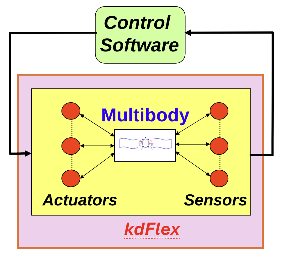
Integration of multibody dynamics with component models in closed-loop simulations#
kdFlex supports the
implementation of a library of parameterized models, that can be instanced and
reused across different simulations.
The Karana.Dynamics.StatePropagator and Karana.Dynamics.ModelManager classes supports the development of system
level simulations that combine the multibody dynamics with device and
environment component models implemented using the
Karana.Models.KModel base class. The KModel classes
support custom parameter classes and methods for interfacing with the
multibody dynamics.
The model manager#
A model manager instance can be used as the simulation manager for integrating
the multibody dynamics with instances of component KModel models and
other user defined classes to build up system level simulations. Such
component models can be registered with the model manager for
invocation and execution within the system level simulation.
The model manager class defines the
MMFunctions struct with
registries for methods of different types. The methods in these
registries are invoked at different times in the system level
execution. Thus the
pre_deriv_fns and the
post_deriv_fns
methods are called just before and after respectively
computing the multibody state time derivative. Thus the pre-deriv
methods can be used to set forces etc. that would effect the equations
of motion, while the post-deriv methods can be used to query
information (e.g., inter-body forces) that depend on the solution to the
equations of motion. The
pre_hop_fns
methods are called before an integration step is
taken. These methods can be used to advance any discrete states within
the component models. Other callbacks - including for zero-crossing
condition - are available to further tailor model manager execution.
While users can add methods to these registries directly, a more common
(and recommended) way is to create a KModel component
model subclass (see KModel component models) that has slots for compliant
methods for implementation (see Model methods section). When a model
is registered with the model manager, its methods are automatically
registered with the model manager as well. The model manager will
thus invoke the model’s methods at the correct times and in the correct
order during state propagation.
This model manager design has several features that support the development of complex system level simulations with coupled multibody, device and environment models. Notable features are:
support for specialized
Karana.Models.KModelParamsparameter classes to go hand-in-hand with component models sub-classed from theKarana.Models.KModelclass.support for multi-rate models
support for tailoring the sequencing of method calls for the component models and the multibody dynamics (e.g., actuator force computation methods should be called before the multibody dynamics is evaluated)
ability to create multiple instances of a component model (e.g., one each for a thruster in a bank of thrusters), while allowing custom parameters for each instance.
creating a catalog of such component model classes for reuse across simulations.
run-time activation and deactivation of the component model instances
support for zero-crossing detection to terminate hops exactly when a zero-crossing condition is met.
The MMFunctions with the callback
registries are stored on the
member of the model manager.
The creation and use of the model manager and component models can be found in several of the example scripts including - 2 link pendulum (basic), n link pendulum (procedural) and Slider-crank with loop constraints.
System state#
When using an integrator, the integrator takes ownership of the system
state. This is necessary to accommodate the needs of adaptive step
integrators which often maintain internal histories of the system state
to manage error while propagating the system state. In this perspective,
the multibody system objects and component models serve as compute
engines for computing the state derivative for the integrator to meet
its state propagation needs. Simply changing the multibody system
coordinates is not therefore the way to update the simulation
state. Such a new state has to be set by calling the model manager
setState() method - which also resets
the internal state of the integrator. This method is used in the
beginning to initialize the system state, and can also be used
mid-stream should the need arise.
If setState()
method is called mid-stream to set a new simulation time, the model manager
will attempt to reschedule all timed events appropriately (see
Timed events section). This means, it will attempt to find the next
time after the new time that a timed event should be executed. However,
since timed events can have non-uniform execution times via the
register_fn, it is impossible to capture all corner cases. Hence, this
should be used with caution when modifying time mid-stream with
non-uniform timed events.
As a reminder, the system state vector is the concatenation of the Q
generalized configuration coordinate values and the U generalized
velocity coordinate values for the coordinate object objects such as
physical subhinge and physical modal body deformation coordinates in the multibody
system. The state vector defines the current independent positions and
velocities that fully describe the system’s kinematic state at any given
moment. A subtle issue of note in this context is the use of global
and local coordinates at the physical subhinges level. As discussed earlier
in the Pose representations section, physical subhinge such as the
SphericalSubhinge use local coordinates centered around local charts to get around the
singularities associated with minimal-coordinate attitude
representations. As a consequence, the numerical integrator state also
makes use of the local coordinates for the physical subhinge. However, to
shield external users from having to deal with this under-the-hood
issue, the
setState()
method always expects the physically meaningful, and
unambiguous, global coordinates when resetting the system
state. Coordinate sanitization is automatically performed at the end of
each integration step, and subhinges may re-center their local charts to
convert the new global coordinate values into local coordinates as
needed.
Tracing/debugging#
The model manager has a trace_state_propagator variable that can
used to enable trace messages for the model manager. This can be very
helpful when debugging model manager-related and model-related issues. To
get enable messages, set trace_state_propagator to True and
ensure the logger where you want to see the messages has a verbosity set
to at least the TRACE level. In
addition, the CallbackRegistrys in have a
trace_callback_registry variable that
can be used to enable trace messages for each
CallbackRegistry. To
enable the messages, set trace_callback_registry to True for
each CallbackRegistry you
want to see messages for, and ensure the logger you want to see messages
on has a verbosity set to at least the TRACE level.
Linearized state space models#
Since multibody dynamics models are nonlinear, so are the system level
models. Designing controllers for such systems with nonlinear models is
challenging. While there is a rich methodology for developing
controllers for linear systems, this is not the case for nonlinear
systems. Control system design and analysis therefore often rely on
linearized state space models for control system design and frequency
domain analysis (including creation of Bode plots). For nonlinear
systems, linearized state space models at specific system configuration
set points are utilized to support the control system design and
analysis workflow. Towards this, there is built in support in kdFlex
for creating linearized state space models from such
model manager system level models for user specified
sets of inputs and outputs about any configuration set
point.
The Karana.Dynamics.Algorithms.stateSpaceGenerator() method can be
used to create a Karana.Math.StateSpace instance for a specified set
of inputs and outputs. The
generate()
can then be called on this object to linearize the system
and compute the state space A, B, C, D matrices. Since the state space
representation is generated using linearization, its values are only
valid in a small neighborhood of the configuration used to do the
linearization. Additionally, such linearizations are typically
meaningful only when the system is in a state of equilibrium, i.e. the
accelerations are near zero. Thus, an equilibration step may be needed
prior to state space model generation.
Such linearized system based control-system design and analysis is complemented with more complete and thorough checkouts in closed-loop time-domain simulations with the full high-fidelity nonlinear model as described in the System level models section.
KModel component models#
Simulation models provide a structured way to interact with objects in
the simulation. For example, they can be used to do things like sense
the position and velocity of a joint or a sensor node, apply forces via
a joint or actuator node, or other tasks such as data logging. The model manager class provides an API for registering such component models so
that their methods and functionality can be included in the overall
system dynamics.
At the C++ level, the component models are created by deriving from a
templatized Karana::Models::KModel class. All of the
template arguments except the first indicate the types of states,
parameters, etc. that the model has. The first template argument is the
model class itself. The remaining template arguments are derived from
specific other classes, e.g., the second template argument must be
derived from Karana::Models::KModelParams, the third from
Karana::Models::KModelScratch, etc.
The diagram below shows the most complex KModel, one that utilizes all the template arguments. Each of these will be discussed in detail in the sections below.


This diagram just uses preHop and preDeriv as some example methods MyModel
may define. See the Model methods section below for more
details. In many cases, not all of the template arguments will be
needed. The default template arguments start with “No”, e.g.,
NoParams, to indicate they are
not used. For example, suppose we had a model that just used discrete
states. Then, the diagram would look like this:


Notice that No* is used to indicate that the model does not have any params or scratch. The NoContinuousStates is not needed at the end, since not specifying this argument will pick up the default (which is NoContinuousStates). When specified in this way, the params, scratch, and continuous_states members will all be nullptrs.
Model methods#
Their are six different methods a user can define in a model that will
run at various points during the simulation. The user does not need to
define all six methods, but must define at least one of them. A model
can skip the implementation of unneeded methods. The model’s
preDeriv and
postDeriv methods will
run before and after the multibody derivative, respectively. The
preHop and
postHop methods will run
before and after each simulation hop, respectively. The preModelStep
and postModelStep step methods will run before and after each of the
model’s steps, respectively. The contents of these methods are
model-dependent, and up to the model writer to define.
The preDeriv and
postDeriv methods are
called at times dependent on the integrator type. The
Karana.Models.SpringDamper.preDeriv() is an example
implementation of the preDeriv method. The preHop and postHop methods will be called at each hop
on the timeline determined by the scheduler. The
Karana.Models.SyncRealTime.preHop() method is an example of a
preHop method, and the
Karana.Models.UpdateProxyScene.postHop() method is an example
of a postHop method.
Environment interaction models, such as gravity, do not have a
pre-determined step size that they need to run at. However device models
often do have specific rates that they need to run at based on the
hardware design. The multi-rate step size can be specified for such
models. The preModelStep and postModelStep methods will run at rates
specified by the model’s multi-rate step size. Model step sizes fall
into one of two categories: uniform and non-uniform. Uniform model steps
are the most common and are step sizes defined by a constant period. For
these models, simply use the KModel setPeriod() method to set the model’s
period. Non-uniform models can use the nextModelStepTime method to define their
non-uniform rate. This method takes as input the current time and
outputs the next time at which the model should step. The
Karana.Models.DataLogger.postModelStep() is an example of a
postModelStep step
method implementation.
Model parameters#
Oftentimes, models utilize parameters in their calculations. For
example, a spring damper model may have the spring constant and damping
value as parameters. In order to define parameters for your model,
create a parameter class that is derived from
Karana::Models::KModelParams and contains the parameters
you want. Then, set the params member variable for the model equal to
a ks_ptr instance of this class during the model’s construction or in
its create method. Model parameter classes should also override the
isReady
method. This method should contain logic to verify that the derived
parameter class’s parameters have been initialized. For parameters that
are real numbers or math objects such as vectors or matrices, see
Math for details on handling of not ready
values. The isReady method will be invoked
automatically for all registered models as part of the overall
simulation initialization. It will be able to flag any not ready
parameters for the model instance. This check will help verify for
anyone creating an instance of the KModel that they have not
accidentally skipped the initialization of all the necessary parameters.
Model scratch#
Sometimes, it is useful to store intermediate results in a model for debugging purposes. The Karana::Models::KModelScratch class gives one a place to store such information. To use it, create a class that is derived from KModelScratch and add class members for the scratch values the model should store. This can be accessed using the scratch member on the model itself. The scratch value should be initialized when the model is created, either in the constructor directly or in the create method.
Discrete states#
Models may have discrete states (states that should not be integrated, but need to be stored and updated as time progresses). Examples of discrete states are the on/off state of a valve or PID integral gain, where the PID model is keeping track of the integrated error separate from the model manager’s integrator, e.g., the model is using an Euler integrator with a fixed step set by the model period. The Karana::Models::KModelDiscreteStates class gives one a place to store such information. To use it, create a class that is derived from KModelDiscreteStates and add class members for the discrete states the model needs to store. This class can be accessed from the discrete_states member of the model itself. The discrete_states value should be initialized when the model is created, either in the constructor directly or in the create method.
Discrete states should be updated by the model in one of the following methods:
These methods run at the hop-boundaries. The method used to update the
discrete states is model dependent. Models that need to update states at
a rate set by the model should use either preModelStep or postModelStep. Models that need to update
their state more frequently e.g., whenever there is a “good” state,
should use the preHop or
postHop methods. A
“good” state refers to one that the integrator will keep, as opposed to
states in the preDeriv
and postDeriv method
that might represent states where an adaptive integrator has taken too
large of a step and will be rolled back. Using the pre* vs. post*
methods is also model dependent. The pre* methods run first, and so
are a good choices when one wants to update a state immediately when a
command comes in, e.g., turning on power or opening a valve. The
preHop method does not
know the exact hop size. It has the intended hop size, but this may be
modified by zero-crossing events, so if the true hop size is needed,
then the postHop method
should be used over the preHop method. The preModelStep and postModelStep do not have this same issue,
as their size is set by the model and not modified by zero-crossing
events.
Continuous states#
Models may have continuous states (states that should be part of the model manager’s integrator). Examples of continuous states are values used to
calculate noise in an IMU model or values used to calculate fuel burned
in a thruster model. The model’s continuous states must be expressible
as a vector of doubles (a km::Vec in C++ or numpy.array in
Python). To use continuous states, derive a class from
Karana::Models::KModelContinuousStates and override the
getX,
setX, and
getdX
methods. These retrieve the current continuous states from the class,
set the continuous states for the class, and retrieve the derivatives of
the continuous states from the class, respectively. All of these methods
make use of Eigen::Ref at the C++ level, so they should be calculated
and stored on the class itself, and an Eigen::Ref returned from them
if the model is a C++ model.
The continuous state derivatives should be updated in either the preDeriv or postDeriv methods. A method at the derivative level must be used, as these are used by the integrator to propagate the state forward in time. The preDeriv runs before the multibody dynamics and the postDeriv runs after the multibody dynamics. The method used by a model often depends on whether the continuous state derivatives need updated multibody dynamics values or not.
Registering and unregistering models#
To affect the simulation, models must be registered with a
model manager. It is recommended that when one writes a model they add a ModelManager.registerModel call in the model’s create method (or the __init__ method if it is a Python model) so that this is done automatically. The model manager
will run the model’s methods at the appropriate times. At any time,
models can also be unregistered from the
model manager. This will effectively disable the
model. To register or unregister a model, simply use the
model manager registerModel() or
unregisterModel() methods,
respectively. This provides a convenient way of activating and
deactivating models at run-time in response to simulation mode
changes.
C++ base class#
The KModel base class in c++ utilizes the curiously
recurring template pattern. This pattern allows the base class to detect
which methods a derived model class has defined. This provides a way to
register only the methods that a user has defined for a model with the
model manager when registering the model. In addition, it also provides other conveniences, such as the params, scratch, etc. member variables’ types matching the derived model’s class’ types.
// Params class for MyModel
class MyModelParams : public Karana::Models::KModelParams {
  public:
    // Override the `isReady` method
    bool isReady() const final;

    // Include parameters here
    float: my_param
    ...
};

class MyModel : public Karana::Models::KModel<MyModel, MyModelParams> {
    // Define methods for the model such as `preDeriv` or `postModelStep` here
    ...
};
The diagrams at the beginning of the KModel component models section show some other examples of using the templated KModel class.
Python base class#
The Karana.Models.KModel bass class in Python compares derived methods with their base class counterparts to determine whether those methods have been overridden or not. Adding params, scratch, discrete states, and continuous states is done by populating member variables in the constructor. The typing for these members (params, scratch, discrete_states, and continuous_states) is provided by a generic in the base KModel class. Similar to C++, the No* versions should be used if the member will not be used. The Python versions of these classes are similar to the C++ with one exception; the KModelParams class is defined from DataStruct, so the parameters can be defined with type hints (that are verified at runtime) by adding them as one would do with any other DataStruct.
# Params class for MyModel
from Karana.Models import KModelParams, KModel, NoScratch, NoDiscreteStates, NoContinuousStates
class MyKModelParams(KModelParams):

    # Override the `isReady` method
    def isReady()-> bool:
        ...

    # Include parameters here
    my_param: float
    ...

class MyModel(KModel[KModelParams, NoScratch, NoDiscreteStates, NoContinuousStates]):
    def __init__(self, name: str, sp: ModelManager):
        super().__init__(name, sp)
        self.params = MyKModelParams(f"{name}_params")
        sp.registerModel(self)

    # Define methods for the model such as `preDeriv` or `postModelStep` here
    ...
Debugging#
Every KModel has a debug_model boolean member variable. This variable is used to enable/disable debug messages for the model. When running a simulation, to get debug messages for a particular model, one should ensure they have a logger whose verbosity is set to at least the debug level and then set the debug_model member variable to true.
To instrument models with these messages, in C++ use
if (debug_model) [[unlikely]] {
    double my_var = someLongFunction();
    stdDebugMsg(std::format("my_var is : {}", my_var);
}
and in Python use
if self.debug_model:
    my_var = someLongFunction()
    self.stdDebugMsg(f"my_var: {my_var}")
KModels and associated classes (params, scratch, discrete states, and continuous states) can also override dumpString methods. These methods will be called and combined whenever KModel.dump() is called, which will display an overall dump for the model. In C++, these methods should be overridden like
class M1Scratch : public kmo::KModelScratch {
  public:
    using KModelScratch::KModelScratch;
    double t = 0.0;

    // Example dumpString override. The returned string should utilize the prefix in front of each line.
    // This can be done in a similar fashion for params, discrete states, and continuous states.
    std::string dumpString(std::string_view prefix = "",
                           const kc::Base::DumpOptions * /*options*/ = nullptr) const override {
        return std::format("{}t: {}\n", prefix, t);
    }
};

class M1 : public kmo::KModel<M1, kmo::NoParams, M1Scratch> {
  public:
    // Other model-related code, constructor, etc. here.

    // Example dumpString override for the model
    std::string dumpString(std::string_view prefix = "",
                           const kc::Base::DumpOptions * /*options*/ = nullptr) const override {
        std::string ret = std::string(prefix);
        // Any custom information should go here.
        ret.append(std::format("Dumping model {}\n", name()));

        // Call the parent method. Here, we add a "    " to the prefix to tab over
        // everything the parent adds relative to the statement we just printed above.
        // The parent method will take care of calling the dumpString methods for the
        // params, scratch, discrete states, and continuous states if appropriate.
        ret.append(kmo::KModel<M1, kmo::NoParams, M1Scratch>::dumpString(
            std::format("{}    ", prefix)));
        return ret;
    }
};
Similarly, in Python, these methods can be overridden like
class M1Scratch(KModelScratch):
    def __init__(self):
        super().__init__("scratch")
        self.t: float = 0.0

    def dumpString(self, prefix: str = "", options: DumpOptionsBase | None = None) -> str:
        return f"{prefix}t: {self.t}\n"

class M1(KModel[KModelParams, M1Scratch, M1States, KModelContinuousStates]):
    # Other model-related code, constructor, etc. here.

    def dumpString(self, prefix: str = "", options: DumpOptionsBase | None = None) -> str:
        # Add our own custom dumpString line. Then, call the parent method with a tab added
        # to the prefix. The parent method will take care of calling the params, scratch,
        # discrete states, and continuous states dumpString methods if appropriate, and the
        # extra tab added to the prefix will tab them over relative to the custom line we
        # added here.
        return f"{prefix}Dumping mode {self.name()}\n" + super().dumpString(
            prefix + "    ", options
        )
KModel DataStructs#
In order to serialize/deserialize a KModel, it must have an associated DataStruct: see DataStruct for details. If the model has parameters, a DataStruct will also need to be created for its parameters, and the parameter DataStruct model should be nested in the KModel’s DataStruct, i.e., the parameter DataStruct should be a field of the KModel DataStruct.
The KModel DataStruct should be derived from KModelDS and override the toModel method. The toModel method is the method that creates a KModel instance from the DataStruct. In some cases, this method will need other simulation objects, e.g., Nodes or PhysicalBodys, used by the KModels constructor. The toModel has a MultibodyDS as an argument that is used for this purpose. The IdMixin.getObjectsCreatedById static method can be used to link IDs used by a DataStruct to object instances in the current simulation. To utilize this, the KModel’s DataStruct should contain fields for the IDs of the objects it needs during construction.
As an example, consider the portion of SpringDamperDS shown below. This model uses two nodes in its constructor. The IDs of these nodes are saved as fields in the DataStruct. Then, they are used in the toModel method to find the actual node objects.
class SpringDamperDS(KModelDS[SpringDamper]):
    """DataStruct for SpringDamper model.

    Parameters
    ----------
    n1 : int
        ID of the first node of the spring damper.
    n2 : int
        ID of the second node of the spring damper.
    params : SpringDamperParamsDS
        Parameters for the SpringDamper model.
    """

    n1: int
    n2: int
    params: SpringDamperParamsDS

    def toModel(self, mm: ModelManager) -> SpringDamper:
        """Create a SpringDamper model instance from this SpringDamperDS.

        Parameters
        ----------
        mm : ModelManager
            The ModelManager to associate this model with.

        Returns
        -------
        SpringDamper
            An instance of the SpringDamper model.
        """
        # Find the nodes needed for the model by ID
        dark = IdMixin.getObjectsCreatedById(self.n1)
        if dark is None or len(dark) != 1:
            raise ValueError(
                f"Could not find unique object associated with original node 1. Found {dark} for node {self.n1}."
            )
        else:
            n1 = dark[0]

        dark = IdMixin.getObjectsCreatedById(self.n2)
        if dark is None or len(dark) != 1:
            raise ValueError(
                f"Could not find unique object associated with original node 2. Found {dark} for node {self.n1}."
            )
        else:
            n2 = dark[0]

        # Create the model
        model = SpringDamper(self.name, mm, n1, n2)
        self.params.setParams(model.params)
        if self.period > 0:
            model.setPeriod(self.period)

        # Keep track of objects created from this DS
        self.addObjectFromId(model)

        return model
In addition, the KModel itself should define the toDS method. The “Karana/SOADyn/pybind11KModel.h” file includes helper methods to create these in pybind11 code. For example, see the excerpt from GeneralKModels_Py.cc below.
#include "Karana/SOADyn/pybind11KModel.h"

// This macro must be called before the associated `addToDSMethod` is called.
// This creates the appropriate type caster.
ADD_TO_DS_METHOD_CASTER(SpringDamper, Karana.Models.GeneralKModels_types, SpringDamperDS)

PYBIND11_MODULE(GeneralKModels_Py, m) {
    // Define SpringDamper class for pybind11 like any other class
    ...

    // Add the toDS method using the helper
    kd::addToDSMethod<SpringDamper>(
    PySpringDamper, "SpringDamper", "Karana.Models.GeneralKModels_types", "SpringDamperDS", "fromModel");
}
Time-domain simulations#
The primary requirement for time-domain simulations is the accurate propagation of the system state, kdFlex supports this primary objective while also accommodating several other important simulation requirements such as:
support for integrating multibody dynamics with component device and environment interaction models
support for using multi-rate models within the system simulation
support for terminating integration steps at zero-crossing boundaries
support for modeling arbitrary time delays
support for step validation and rollback
support for handling discrete, discontinuous run-time changes to system dynamics
support for activating and deactivating component models at run-time
scheduling and registering of arbitrary timed events during a simulation run
support for the use of different types of multibody dynamics solvers
support for accurate and high order numerical integrators as needed, including variable-step and stiff integrators
providing deterministic and unambiguous handling of time representations
support verification of parameter initialization across all model instances
support for periodic data logging
support for live updates to visualization and data plots at run-time
fast computational performance for closed-loop simulation use
embeddable for hardware-in-the-loop simulations
The state propagator class
supports these features required for the development of
realistic and complex system level time-domain simulations.
Numerical integration#
For time-domain simulations, the class supports the instantiation of a
Karana.Math.Integrator numerical integrator from a large suite of
fixed and variable step integrators for time domain state propagation
and simulation. The integrator options range from the fixed step
Karana.Math.EulerIntegrator Euler 1-step integrator and the fourth
order Karana.Math.RK4Integrator integrators, to the
Karana.Math.CVodeIntegrator and Karana.Math.ArkExplicitIntegrator
large family of variable step integrators from Lawrence Livermore’s
SUNDIALS numerical
integrator suite.
The state propagator#
The state propagator class is derived from the model manager class and adds the
functionality for propagating the model manager state in time using
numerical integrators.
State propagation hops#
The state propagator
advanceTo() method can be used to request the advancement of the
system state over time for a simulation scenario. Such a time
advancement request is broken up by the state propagator into discrete
state propagation time intervals referred to as time hops. The
different call rate times of the component models are used to determine
the (irregular) time hop sizes required to meet the overall
propagation time barrier requirements. The numerical integrator
propagates the system state across individual hops by using the state
propagator to orchestrate calls to the methods of the registered
KModel component models and the multibody dynamics in the correct
order to compute the state derivatives.
Zero-crossings#
In addition to this normal state propagation process, the state propagator also
has support for zero-crossing detection. This phrasing is used for
situations where a simulation hop is required to terminate when an
implicitly defined, state dependent, condition is met.
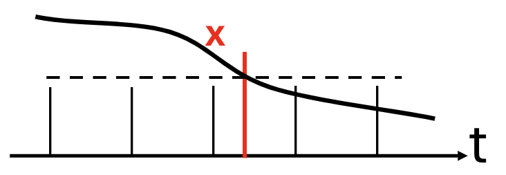
Terminating time hops at zero-crossing events#
Examples of this are body collision events, state-dependent triggers etc. When a zero-crossing condition method is registered with the state propagator, the propagator will monitor these zero-crossing conditions, and when triggered, will use a regula-falsi iteration to find the precise time boundary when the condition triggered to terminate the hop, execute appropriate registered actions before proceeding on to the next hop.
Timed events#
The state propagator also allows the registering of user defined
Karana.Dynamics.TimedEvent instances along with associated custom
handlers. The time event executions can be one time, irregular, or
periodic. The state propagator will ensure that hops terminate at the
registered time boundaries for such timed events to invoke their
associated handlers. Examples of use of timed events are for simulation
needs such as data logging, updating visualization etc. This flexible
capability allows user to incorporate arbitrary events into their
simulations.
kdFlex uses numpy.timedelta64 nanosecond precision class for time (Karana::Math::Ktime at the C++ level). Its
use avoids any ambiguities that can occur from double precision
representations of time.
Geometry Layer#
Scene layer#
kdFlex defines an abstract interface for working with 3D geometries
attached to the physical physical bodies in the multibody system. This
abstract interface and its various implementations make up the
Karana.Scene.Scene Scene layer. kdFlex provides various scene
implementations for different purposes and third-party backends. For example,
Karana.Scene.WebScene is a scene implementation that provides a
live 3d visualization of the simulation in the web browser using
three.js. Karana.Scene.CoalScene implements
the same scene interface for collision detection using
Coal. This architecture is
extensible and allows the addition of new backend scenes by simply
implementing new specializations of the scene class.
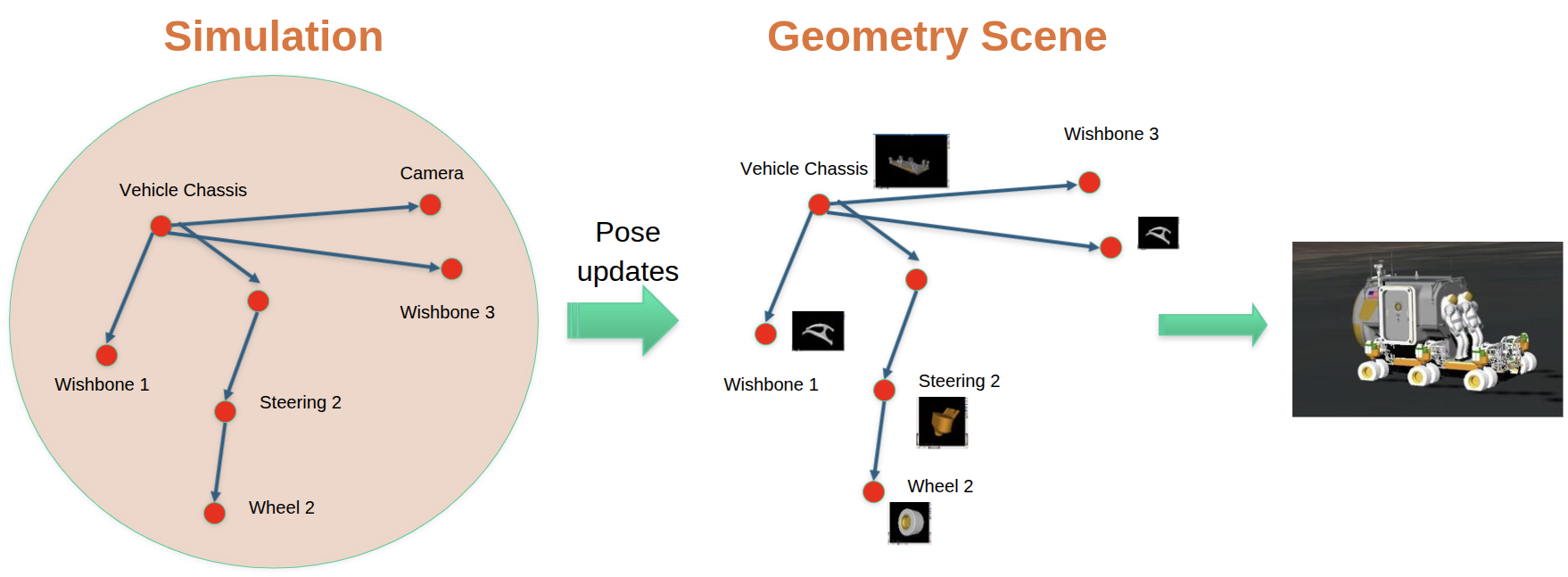
Updating of visualization scene from simulation data#
ProxyScene#
There is often a need for multiple scene instances
in a single simulation - for example the need for both collision detection and 3d
graphics. Karana.Scene.ProxyScene is a scene
implementation that manages other scene implementations. The multibody and
other multibody classes by and large interface and interact with the
proxy scene manager class, and use it to mediate the
interactions with the registered scene backends. We refer to Scene
implementations managed by proxy scene as client
Scenes. In addition to synchronizing state across client Scenes,
proxy scene also acts as a bridge between the frame
and scene layers. That is, proxy scene
uniquely supports attaching objects from the Scene layer to Frames from
the Frame layer. The upshot is, as a frame moves, the
proxy scene will correspondingly move attached geometries
in all of the client Scenes.
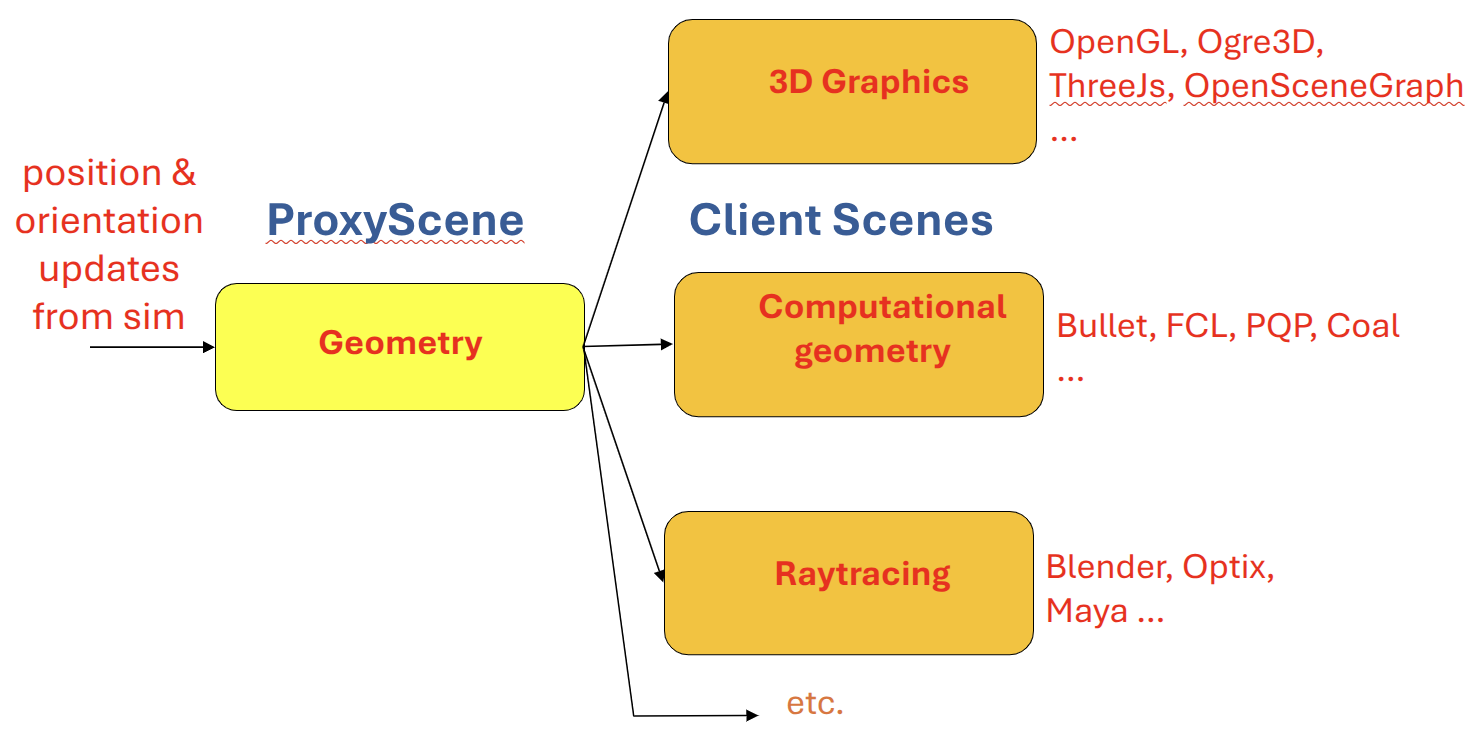
ProxyScene interface to client Scenes#
A typical setup in a full simulation will look like this:
Create a
Karana.Dynamics.MultibodyCreate a
proxy sceneCreate Scene objects in the
proxy sceneinstance, and attach them tophysical bodiesand other framesCreate various client Scenes as needed and register them using the
proxy sceneregisterClientScene()method.
This order doesn’t need to be strictly adhered to. It’s also reasonable to
populate the Karana.Dynamics.Multibody and proxy scene in tandem, creating each body and its
attached geometries simultaneously. A client scene can also be registered at
any time. proxy scene immediately syncs up a newly registered client scene and
continues to update the client scene with any further changes.
As a simulation evolves and a frame moves around, proxy scene will
need to be told when to update the corresponding transforms in its
client Scenes. To sync a client scene’s transforms with the Frame
layer, call the proxy scene
update()
with the client Scene in question as an argument. To update
all client Scenes, just call update()
with no arguments.
Each Karana.Scene.ProxySceneNode and Karana.Scene.ProxyScenePart
implementation in proxy scene has a corresponding
scene node and scene part implementation in each client scene
which should be used exclusively with that client Scene. In most cases,
where proxy scene is managing the Scene layer, this means
creating instances of proxy scene node and
proxy scene part to populate the ProxyScene (and
consequently all of the client Scenes).
Scene objects#
Each scene is a container for instances of Karana.Scene.SceneNode
and Karana.Scene.ScenePart.
Each scene node has a Karana.Math.SimTran, which consists of a
position, rotation, and uniform scale factor relative to a parent. scene node instances
may be attached to one another with attachTo(), giving the overall Scene a tree
structure (with an implicit root node). Each scene node also has a visibility flag, which can be used to hide the node and all of its descendants.
A scene part is a scene node
that additionally has a 3D geometry, which can either be a primitive
shape such as a sphere or cylinder, or a triangular mesh. A
scene part also has a material describing its surface properties and
appearance.
Typically a scene will consist of a tree, where branches are scene node instances, and leaves are scene part instances.
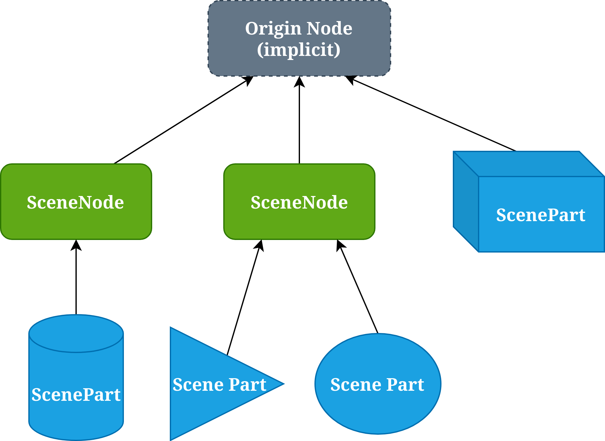
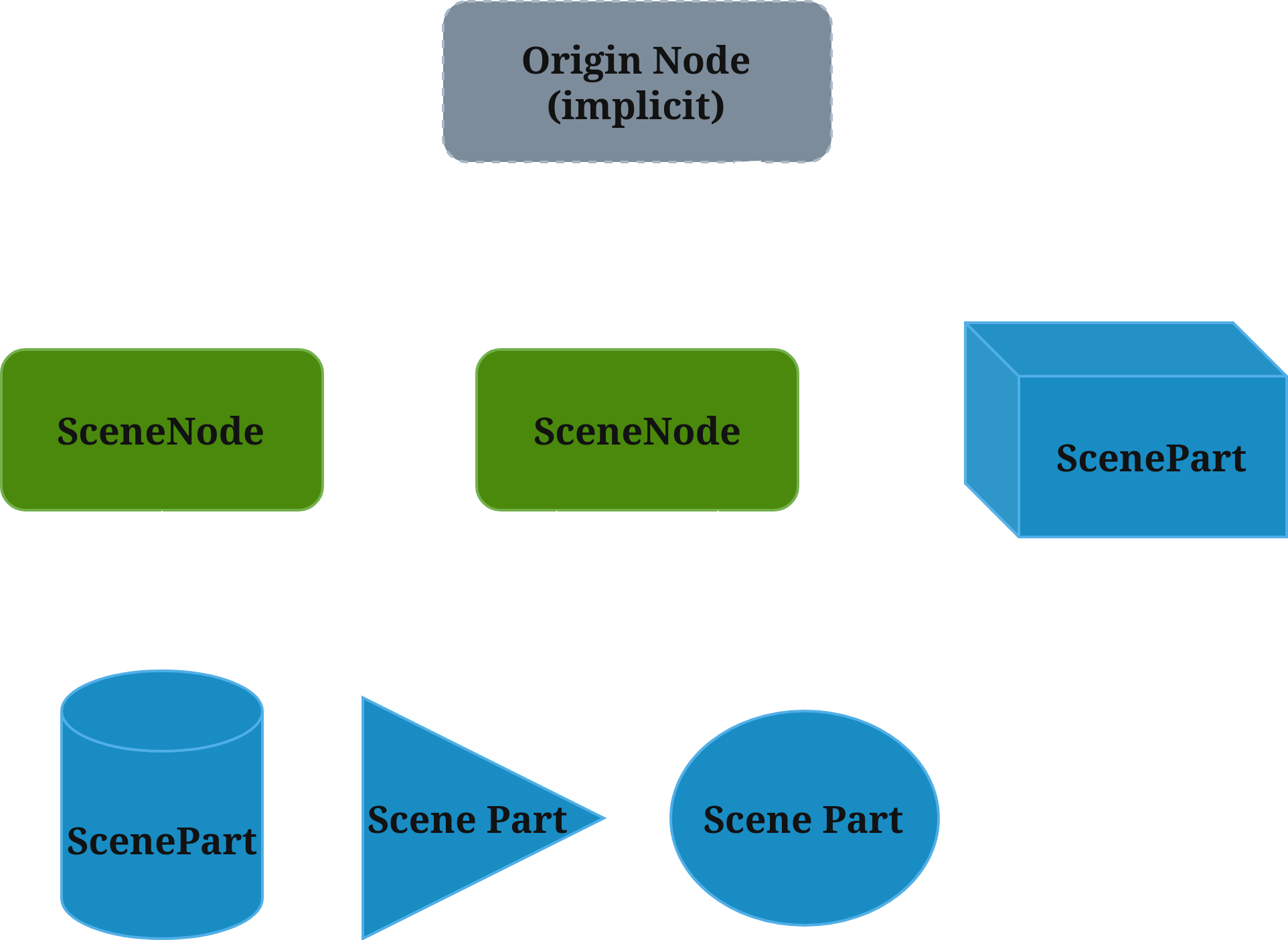
Geometries#
Each scene part has a Karana.Scene.AbstractStaticGeometry defining its 3D shape. A geometry may be an analytical primitive shape (e.g., Karana.Scene.BoxGeometry, Karana.Scene.SphereGeometry), or a triangular mesh (typically Karana.Scene.StaticMeshGeometry).
Creating a scene part requires a VarStaticGeometry, which is a variant that can be a shared pointer to any of the geometry types defined in kdFlex:
Additional user-defined geometry types can also be used by first upcasting to Karana.Scene.AbstractStaticGeometry.
The same geometry instance may be passed to multiple scene part instances for easy geometry instancing.
Materials#
Each scene part also has a material. There are currently two choices for material type:
Karana.Scene.PhysicalMaterial: this is a conventional PBR material with fields such as base color, metalness, and roughness.Karana.Scene.PhongMaterial: this is commonly used material with fields for diffuse, specular, emissive colors and textures.
Creating a material is a two-step process. First, create a corresponding info Karana.Scene.PhysicalMaterialInfo or Karana.Scene.PhongMaterialInfo, and update its fields as desired. Then to create the actual material, pass the info instance into the material’s create method.
Creating a scene part requires a VarMaterial, which is a variant that can be a shared pointer to either material type.
A part’s material may be modified at any time by calling setMaterial() to assign a new material instance to the part.
Layers#
Each scene part belongs to layers. Layers are implemented using a layer_t which is a 32-bit unsigned integer, where each bit represents a different layer that a scene part may inhabit. Scene parts may then be filtered using a layer_t bitmask, such that a part is filtered out if it doesn’t have any layers in common with the bitmask.
The least significant twenty-four bits are set aside for user defined layers and will not be used internally by kdFlex. For convenience kdFlex defines the constants Karana.Scene.LAYER_CUSTOM0 through Karana.Scene.LAYER_CUSTOM23, which are simply the first twenty-four powers of two.
The most significant eight bits are reserved for layers defined by kdFlex, with constants Karana.Scene.LAYER_RESERVED0 through Karana.Scene.LAYER_RESERVED7. kdFlex currently makes use of the first four reserved layers:
Karana.Scene.LAYER_PHYSICAL_GRAPHICS: reserved for visualization of real, physical objectsKarana.Scene.LAYER_ORNAMENTAL: reserved for visualization of ornamental objects not suitable for sensor simulationKarana.Scene.LAYER_STICK_FIGURE: reserved for scene parts generated bycreateStickParts()Karana.Scene.LAYER_COLLISION: reserved for parts used for collision detection
kdFlex also defines several layer sets:
Karana.Scene.LAYER_NONE: no layers, that is, the number zero.Karana.Scene.LAYER_ALL: all layers, that is, the maximum 32-bit unsigned integer.Karana.Scene.LAYER_PHYSICAL: combination ofLAYER_PHYSICAL_GRAPHICSandLAYER_PHYSICAL_COLLISION. This may be useful if the same geometry is suitable for both graphics and collision detection.Karana.Scene.LAYER_GRAPHICS: combination of all reserved graphical layers (LAYER_PHYSICAL_GRAPHICS,LAYER_PHYSICAL_ORNAMENTAL,LAYER_PHYSICAL_FIGURE). This is the default bitmask used for visualization.
Filtering based on layers is done in two places:
ProxyScene.registerClientScenetakes alayer_targument, defaulting toLAYER_PHYSICAL_ALL. This can be used to filter which scene parts should be implemented in a registered client scene.Client scenes may filter parts, depending on the application. For example,
Karana.Scene.GraphicalSceneCamerahas alayer_tbitmask controlling which layers should be rendered (defaulting to {py:const}`Karana.Scene.LAYER_GRAPHICS).
Uniform and intrinsic scale#
Each scene node has a Karana.Math.SimTran, which
includes a scale factor relative to the node’s parent. This can be used
to scale entire subtrees within a scene. The scale factor is uniform,
meaning it is a scalar applied in all three directions. Without this
limitation it would be possible to introduce skew by chaining together
rotations and non-uniform scaling transforms, which is problematic for
many scene backends.
To support non-uniform scaling, the scene part class has the
notion of intrinsic scaling. The intrinsic scaling can be non-uniform,
and is only applied directly to the part and is ignored when computing
the world transform for any descendant parts. A part’s intrinsic scale
can be accessed through the getIntrinsicScale and
setIntrinsicScale
methods.
Importing assets#
Scene assets such as geometries and materials are often created offline
and need to be loaded from files. kdFlex defines an abstract
interface Karana.Scene.AbstractImporter and implementation
Karana.Scene.AssimpImporter, which can be used to load asset
files into native kdFlex types. To load a file, first create an
AssimpImporter instance, then invoke the importFrom method with a filepath argument. This
returns a Karana.Scene.ImportResult containing any assets
found in the given file.
There are multitude of widely used file formats, whose contents may
range from a single asset to an entire serialized scene, so the
ImportResult may consist of any number of assets in general.
Parts managed by a multibody#
Scene parts attached to a physical body should preferably be managed
by the body by calling PhysicalBody.addScenePartSpec. The
Karana.Scene.ScenePartSpec argument is a plain struct with
all of the information needed to eventually create a scene part. This has a number of benefits:
The scene part’s lifetime is automatically managed by the body
The scene part can be specified immediately while deferring its creation until a
proxy sceneis registered with the multibody viasetScene.The scene part will be included when serializing the multibody
Visualization#
kdFlex provides a Scene implementation for 3d visualization called
Karana.Scene.WebScene. Karana.Scene.WebScene is implemented on top
of three.js, and uses WebGL to do hardware
accelerated 3d-rendering in the web browser. This makes it possible to
bring up a live, interactive visualization of a simulation on a remote
machine by simply opening the correct URL in a web browser. kdFlex also
comes with a standalone electron
application that can be used for local 3d visualization in lieu of the
web browser option.
In most cases, where proxy scene is managing the scene layer,
graphics can be enabled by creating the Karana.Scene.WebScene client
scene and registering it via proxy scene
registerClientScene().
This will automatically populate the
Karana.Scene.WebScene client with whatever geometries have been set up
in proxy scene.
WebUI#
To instantiate Karana.Scene.WebScene, first create an instance of
Karana.WebUI.Server, which manages communication between the
simulation process and any number of connected front-end
clients. Karana.WebUI.Server accepts connections on a port specified
at construction time and queryable by calling
Karana.WebUI.Server.port().
To open a browser-based front-end, simply enter the URL to access the port over
http. For example, if Karana.WebUI.Server.port() returns 9090 and the
simulation is running locally, enter http://localhost:9090 in your web
browser’s address bar. If the simulation is running on a remote machine,
replace localhost with an IP address or domain that resolves to the simulation
server. It’s not always possible for Karana.WebUI.Server to know how you will
be accessing it, but Karana.WebUI.Server.guessUrl() returns a best-guess URL
string.
To open the standalone front-end for a locally running simulation, call
Karana.WebUI.Server.launchLocalClient(). This launches an electron
application on the same machine as the simulation that automatically connects
to the simulation server.
The Visualization notebook provides an example of using the kdFlex visualization capability .
Collision dynamics#
Collision detection is handled by collision engines. These detect whether objects are colliding, and provide information like the penetration of the collision and the collision normal. The Karana.Collision.FrameCollider class is a generic way to capture the information coming from collision engines. Once this information is gathered, contact forces can be calculated from it. The Karana.Models.PenaltyContact model passes the information from the FrameColliders to classes derived from Karana.Collision.ContactForceBase: these are the classes which calculate and apply the contact forces. The diagram below illustrates the flow of data graphically:


Each of the pieces of this pipeline are explained in detail in the subsections below.
Collision engines#
Currently, Karana.Scene.CoalScene is the only collision engine that comes
packaged with kdFlex. However, more may be added in the future.
Karana.Scene.CollisionScene is an extension of scene that adds a
more specialized interface for querying collisions that can be fed back
into the simulation for contact dynamics. Karana.Scene.CoalScene is
built upon the Coal project that
implements Karana.Scene.CollisionScene. In most cases, where
proxy scene is managing the Scene layer, collisions can be enabled by
creating a Karana.Scene.CoalScene client scene and registering it via
proxy scene
registerClientScene().
This will automatically populate the CoalScene
client with whatever geometries have been set up in proxy scene.
FrameCollider#
The Karana.Collision.FrameCollider class is a helper that maps
collisions from a Karana.Scene.CollisionScene to the frame
layer. Karana.Collision.FrameCollider.collide() sweeps through the
Karana.Scene.CoalScene and invokes the registered callback for each
pair of contact points between frames due to their attached
geometries. This process provides a pathway for returning information
and invoking simulation level actions based on events triggered in the
collision client scenes.
To ignore collisions between frame pairs, call the
FrameCollider.ignoreFramePair method. In many cases a
multibody model may have overlapping geometries between which collisions
must be ignored. The convenience method
FrameCollider.ignoreAllCurrentlyTouchingPairs sweeps
through and ignores all such pairs.
PenaltyContact#
The Karana.Models.PenaltyContact uses
FrameCollider(s) and applies penalty forces to
physical bodies based on their contact penetration, relative velocity, etc.
The PenaltyContact model uses a ContactForceBase class to perform the contact force calculations. This can be any class derived from ContactForceBase. The FrameCollider(s) and ContactForceBase class are all passed as constructor arguments to PenaltyContact. For example, the Karana.Collision.HuntCrossley contact force calculation uses a Hunt-Crossley contact model for normal forces and Coulomb friction for the tangential component. The PenaltyContact can handle collisions coming from multiple sources (multiple FrameColliders).
ContactForceBase#
Every contact force calculation is done on classes derived from ContactForceBase. Derived classes must override the computeForce method. This method receives the Karana.Collision.FrameContact structure for the collision as well as two nodes (one for each body involved in the collision). The computeForce method uses this information to calculate the contact force (as a SpatialVector) and returns it.
Putting it all together#
The steps to add collision detection and contact forces to a simulation are as follows:
Create collision engines. Oftentimes, only one collision engine will be used, but there are scenarios where there may be multiple.
Create a
FrameColliderfor each collision engine.Create a
PenaltyContactwith theFrameCollider(s) andContactForceBaseas constructor arguments.Set parameters for
ContactForceBaseclass if appropriate.
The 2 link pendulum (collisions) example notebook illustrates the use of collision dynamics with kdFlex.
Simulation Core#
DataStruct#
The DataStruct Python class is built upon pydantic ‘s BaseModel and
offers a useful way to define structured data in Python. It catches
typing errors at runtime, which allows for early error detection and
facilitates throwing better exceptions. This helps users efficiently fix
problems. For fundamental usage that overlaps with pydantic.BaseModel,
refer to the pydantic
documentation.
Type Checking and Validation#
DataStruct leverages pydantic ‘s robust type checking, ensuring that
data conforms to defined types at creation and when fields are set. This
allows for early error detection and informative exceptions.
Basic Validation#
One can define fields with specific types and add validation rules using
Annotated and pydantic.Field:
from typing import Annotated
from Karana.KUtils.DataStruct import DataStruct
from pydantic import Field
from pydantic_core._pydantic_core import ValidationError

class A(DataStruct):
    """
    Parameters
    ``````--
    a : int
        Description for a.
    b : str
        b is a string.
    c : Annotated[int, Field(gt=0)]
        Positive integer.
        I'm a long description.
    d : float
        I'm a float.
    """
    a: int
    b: str = "hello"
    c: Annotated[int, Field(gt=0)] # 'c' must be a positive integer
    d: float = 2.2

# This will work fine
a = A(a=3, b="hello", c=4)

# This will fail because 'c' must be greater than 0
# b = A(a=3, b="hi", c=-1)
Validation is also enforced when modifying fields after a DataStruct
instance has been created.
a = A(a=3, b="hello", c=4) # Instance created successfully

# This will fail as the value for 'c' is invalid
# a.c = -1
Custom types and quantities#
Karana.KUtils.Ktyping defines convenient types that utilize the Python
quantities package.
Here’s an example using the Mass (a scalar value that must have units
corresponding to mass) and Length3 (3-vector with units that
correspond to length) types:
from Karana.KUtils.Ktyping import Mass, Length3
from Karana.KUtils.DataStruct import DataStruct
import quantities as pq
import numpy as np
from pydantic_core._pydantic_core import ValidationError

class A(DataStruct):
    m: Mass
    l3: Length3

# These will work (can be floats or quantity objects with compatible units)
a = A(m=3.0, l3=np.zeros(3))
a = A(m=3.0 * pq.slug, l3=np.ones(3))
a = A(m=3.0 * pq.slug, l3=np.ones(3) * pq.mm)

# This will fail due to incompatible units (ft for Mass)
# a = A(m=3.0 * pq.ft, l3=np.ones(3) * pq.mm)
The system also provides custom unit-less types like Vec3 (for
3-element numpy arrays) and Mat33 (for 3x3 numpy arrays), which
include shape and type validation. There are also convenient checks for
use in Annotation, like normCheck, which validates against a specified
norm value and tolerance:
import numpy as np
from typing import Annotated
from Karana.KUtils.Ktyping import Vec3, normCheck
from Karana.KUtils.DataStruct import DataStruct
from pydantic_core._pydantic_core import ValidationError

class V3norm(DataStruct):
    v3: Annotated[Vec3, normCheck(2.5, 1e-5)] # Vec3 with norm ~2.5, tolerance 1e-5

# This passes because the norm (approx 2.5) is within tolerance
a = V3norm(v3=np.array([0.0, 2.5 + 1e-6, 0.0]))

# This fails because the norm (approx 2.5 + 1e-4) exceeds the tolerance
# V3norm(v3=np.array([0.0, 2.5 + 1e-4, 0.0]))
Versioning#
The DataStruct class provides a built-in mechanism for tracking
changes over time using a version field. This allows one to manage
backward compatibility, automatically upgrade older versions if desired,
and flag breaking changes.
The version field is defined as a 2-integer tuple. This tuple
adheres to a common semantic versioning pattern to differentiate between
types of changes.
The first number in the tuple represents the major version. A change
in the major version typically indicates breaking changes that are
not backward compatible. When a major version mismatch occurs (e.g.,
trying to load a 1.x version when the current is 2.x), it usually
necessitates an error, as automatic upgrades cannot be done without user
intervention. For example, suppose there is a DataStruct with a new
field added called new_field with no default. Further, suppose there
is no good way to choose a default for this field for users. In this
case, user intervention is required to choose the right value, and this
is not backward compatible. The major version number should be
incremented, and encountering older versions should trigger an error
with a message or link to documentation that describes what the
new_field is and how users might choose the right value and upgrade
their DataStruct.
The second number in the tuple represents the minor version. Changes
to the minor version are backward compatible. This means that an older
minor version (e.g., 1.1) can often be automatically updated or
migrated to a newer minor version (e.g., 1.2) without data loss or
functional issues. For example, suppose there is a DataStruct that
gains a new field called new_field with a default value of 3.0. This
is backwards compatible as older versions of this DataStruct can just
use the new field with the new default. It is still a good idea to
trigger a warning to users in this case letting them know this is
happening. Furthermore, providing a way for them to upgrade, e.g., add
this new_field and step up the version so they don’t see the warning
again, is helpful. This can often be accomplished by suggesting they use
toFile to save the automatically upgraded version of the DataStruct
to wherever they are currently loading it from.
Setting the current version#
The DataStruct class defines a _version_default class variable
that holds the default version. To set the current, expected version for
a class derived from DataStruct, override this _version_default
class variable.
from Karana.KUtils.DataStruct import DataStruct
from typing import ClassVar

class MyData(DataStruct):
    # Set the current expected version for this data structure.
    # This overrides the (0, 0) default inherited from DataStruct.
    _version_default: ClassVar[tuple[int, int]] = (1, 0)
    # ... other fields
Version validators#
To implement the logic for handling different versions (issuing
warnings, raising errors, or performing automatic upgrades), you should
use Pydantic’s field_validator or model_validator.
A field_validator can validate the version field itself and trigger
warnings or errors. However, a field_validator cannot modify other
variables of the class, so it cannot be used for automatic upgrades.
Below is an example of a field_validator used for version checking and
issuing warnings/errors:
from typing import ClassVar
from pydantic import field_validator
from Karana.Core import error, warn
from Karana.KUtils.DataStruct import DataStruct

class A(DataStruct):
    @field_validator("version", mode="after")
    @classmethod
    def _validateVersion(cls, version: tuple[int, int]) -> tuple[int, int]:
        """Validate the version.
        This cannot modify other variables of the class.

        Parameters
        ----------
        version : tuple[int, int]
            The version.

        Returns
        -------
        version : tuple[int, int]
            The validated version.
        """
        if version == cls._version_default:
            # Early out for most common case where version matches the default.
            return version
        elif version < cls._version_default:
            # Trigger a warning for older, potentially compatible versions.
            warn(
                f"Got version {version} which is less than the current version {cls._version_default}."
            )
        else:
            # Trigger an error for newer, potentially incompatible versions.
            raise ValueError(f"Got version {version} which is greater than the current version {cls._version_default}.")

        # Return the validated version
        return version

# Example usage illustrating the field validator's behavior:
a = A(version=(0, -1)) # This will trigger a warning
b = A(version=(1, 0))  # This will trigger an error
For more complex logic, especially when there is a need to upgrade
other fields based on a version mismatch, one should use a
model_validator. A model_validator gets access to the full model
instance (self), allowing it to modify other fields. This is ideal for
implementing automatic backward-compatible upgrades.
Below is an example of a model_validator that performs automatic upgrades:
from typing import Self, ClassVar
from pydantic import model_validator
from Karana.Core import error
from Karana.KUtils.DataStruct import DataStruct

class B(DataStruct):
    # Suppose this is a newly added field in 1.1 (from 1.0).
    f: int = 3
    g: int

    # This class now sets its _version_default to (1, 1) overriding the (0, 0) default from DataStruct.
    _version_default: ClassVar[tuple[int, int]] = (1, 1)

    @model_validator(mode="after")
    def _validateVersion(self) -> Self:
        """Validate the version.

        This is a model validator, so it gets access to the full model. This can be used to upgrade other
        fields based on a version mismatch.

        Returns
        Self
            self after validation.
        """
        if self.version == self._version_default:
            # Early out if the version matches the current default.
            return self

        if self.version < self._version_default:
            # This block handles backward-compatible upgrades (typically minor version changes)
            # or raises an error for major version downgrades.
            if self.version[0] < self._version_default[0]:
                # If the major version is older, this is considered a breaking change.
                raise ValueError("Major version change. Cannot handle! To upgrade please do <insert steps here>.")
            else:
                # If only the minor version is older, an automatic, backward-compatible upgrade is possible.
                print("Automatic upgrade. Backward compatible. Add a message telling the user this has been done and what to do to avoid this warning in the future.")

                # Do the upgrade. Here our example upgrade sets g = f.
                self.g = self.

        if self.version > self._version_default:
            # Should not get a nonexistent future version. Trigger an error.
            raise ValueError(f"Got version {self.version}, which is a nonexistent future version.")

        return self
Equality and approximate equality (isApprox())#
DataStruct instances support both strict equality checking with the
usual == operator and approximate equality checking via the isApprox
method. These methods recurse through the composite data types, e.g., a
field that is a list of other DataStruct s.
Consider the following example with nested DataStruct instances and
numpy arrays:
from Karana.KUtils.DataStruct import DataStruct
from Karana.KUtils.Ktyping import Vec3
from copy import deepcopy
import numpy as np

class A(DataStruct):
    a: int
    b: str = "hello"
    c: int

class B(DataStruct):
    a: dict[str, list[list[A] | A]]
    a2: dict[str, dict[str, int | tuple[A, A] | Vec3]]

a1 = A(a=3, b="hello", c=4)
a2 = A(a=3, b="hello", c=4)
b1 = B(a={"1": [[a1, a2], a1], "2": []}, a2={"3": {"3.1": 3, "3.2": (a1, a2), "3.3": np.zeros(3)}})

b2 = deepcopy(b1)
b2.a2["3"]["3.3"] += 2e-8 # Introduce a small difference in a numpy array element

# These two differ by 2e-8, so isApprox passes with prec=1e-7
assert b1.isApprox(b2, prec=1e-7)

# These two still differ by 2e-8, so isApprox fails with prec=1e-8
assert not b1.isApprox(b2, prec=1e-8)

# In their current state, b1 and b2 are not strictly equal
assert b1 != b2

# After making b2 a fresh deepcopy of b1, they are strictly equal
b2 = deepcopy(b1)
assert b1 == b2
Saving to and loading from files#
DataStruct provides convenient methods for saving to files, the
toFile method, and loading the data back, the fromFile method. The
file type is determined by the file name’s suffix. Currently, the
supported formats are json, yaml, pickle, and h5.
Custom class handling#
In order to save/load a DataStruct, all fields need to be
serialized. In most cases, a DataStruct ‘s fields will be serializable
without any changes. However, for custom classes, e.g.,
Karana.Math.UnitQuaternion, small modifications need to be
made. Custom classes define certain methods in order to be serialized,
and for yaml and json, must also be registered with the appropriate
saver/loader. The classes in kdFlex that are often used, e.g.,
UnitQuaternion and SpatialVector, already have the methods
defined. If saving/loading from a pickle or h5 file, then nothing
needs to be done, and if saving/loading from yaml or json all one
must do is register them with the appropriate saver/loader.
YAML#
This example shows saving and loading a class that uses UnitQuaternion
and SpatialVector. These classes already have to_yaml and
from_yaml defined, so serialization and deserialization is handled
automatically.
import numpy as np
from Karana.KUtils.DataStruct import DataStruct
from Karana.Math import UnitQuaternion, SpatialVector

class YamlInOut(DataStruct):
    a1: UnitQuaternion = UnitQuaternion(0.5, 0.5, 0.5, 0.5)
    a2: SpatialVector = SpatialVector(np.array([1-3]), np.array([4, 6, 8]))

# Example usage:
dark = YamlInOut()
dark.toFile("example.yaml")
loaded_dark = YamlInOut.fromFile("example.yaml")
assert loaded_dark == dark
For examples of how to write the to_yaml and from_yaml methods, see
Karana.Math._Math_Py.py.
JSON#
This example shows saving and loading a class that uses UnitQuaternion
and SpatialVector. These classes already have to_json and
from_json defined, so serialization and deserialization is handled
automatically.
import numpy as np
from Karana.KUtils.DataStruct import DataStruct
from Karana.Math import UnitQuaternion, SpatialVector

class JsonInOut(DataStruct):
    a1: UnitQuaternion = UnitQuaternion(0.5, 0.5, 0.5, 0.5)
    a2: SpatialVector = SpatialVector(np.array([1-3]), np.array([4, 6, 8]))

# Example usage:
dark = JsonInOut()
dark.toFile("example.json")
loaded_dark = JsonInOut.fromFile("example.json")
assert loaded_dark == dark
For examples of how to write the to_json and from_json methods, see
Karana.Math._Math_Py.py.
Pickle and H5#
To save/load from a pickle or h5 file, the class need only be
picklable. This means that its __getstate__ and __setstate__ must be
defined. Nothing needs to be done on the DataStruct itself, the class
just needs to define these methods.
File I/O Examples#
DataStruct comes pre-loaded with support for numpy arrays and
quantities.Quantity s when saving to and loading from files. Custom
classes can be registered as described above. It also automatically
supports composite types, e.g., embedded DataStruct instances, lists
of dictionaries of numpy arrays, etc.
Here’s an example demonstrating saving and loading an instance of A (a
DataStruct containing Mass and Length3 types) to a YAML file:
from pathlib import Path
from Karana.KUtils.Ktyping import Mass, Length3
from Karana.KUtils.DataStruct import DataStruct
import numpy as np
from tempfile import NamedTemporaryFile

class A(DataStruct):
    m: Mass
    l3: Length3

a = A(m=3.0, l3=np.zeros(3)) # Create an instance

tf = NamedTemporaryFile(suffix=".yaml") # Create a temporary YAML file
p = Path(tf.name)

a.toFile(p) # Save the DataStruct to the file
b = A.fromFile(p) # Load it back

assert a == b # Verify equality
Additionally, DataStruct instances can be saved to and loaded from an
h5py group within an HDF5 file.
import h5py
from Karana.KUtils.DataStruct import DataStruct
from tempfile import NamedTemporaryFile
import numpy as np

class A(DataStruct):
    x: float = 3.0
    y: str = "hi"

class B(DataStruct):
    a3: dict[str, A | int]

# Create a sample B instance
a1 = A(x=1.0, y="1")
b = B(a3={"5": a1, "6": 3})

tf = NamedTemporaryFile(suffix=".h5")
with h5py.File(tf.name, "r+") as f:
    g = f.create_group("new_group") # Create an HDF5 group
    b.toFile(g) # Save the DataStruct to the group
    b_new = B.fromFile(g) # Load it back from the group
    assert b == b_new
NestedBaseMixin#
The NestedBaseMixin provides a way to deserialize nested Pydantic
classes, where the nested class is a base class and subclasses may be
provided, e.g., BodyDS in BodyWithContextDS from
Karana.Dynamics.SOADyn_types. The NestedBaseMixin should be added as
a mixin to the base class (BodyDS in the example with
BodyWithContextDS). The string provided to NestedBaseMixin will be
the name of the field that is added to the base class and all of its
derived classes by the mixin, and it is used to track the actual class
type used. pydantic ‘s SerializeAsAny should always be used when the
NestedBaseMixin is used, so that the correct type is serialized as
well. SerializeAsAny is essentially duck-type serialization as opposed
to strict-type serialization.
Below is an example of how NestedBaseMixin is used:
from pydantic import SerializeAsAny
from Karana.KUtils.DataStruct import DataStruct, NestedBaseMixin

class Base(DataStruct, NestedBaseMixin("type_name")):
    a: int = 3

class D1(Base):
    b: int = 4

class D2(Base):
    c: int = 5

class Test(DataStruct):
    l: list[SerializeAsAny[Base]] = []

t = Test(l=[D1(b=0), D2(c=0), Base(a=1)])

t.toFile("test.yaml")

assert Test.fromFile("test.yaml") == t
To/From DataStruct and Dictionary#
Converting DataStruct instances to and from standard Python
dictionaries is straightforward. To convert a DataStruct instance to a
dictionary, use the model_dump method:
my_dict = my_data_struct.model_dump()
To create a DataStruct instance from a dictionary, use the ``**
dictionary unpacking operator:
my_data_struct = MyDataStruct(**my_dict)
IdMixin#
The Karana.KUtils.DataStruct.IdMixin class is used to track objects that have been created from DataStructs. This associates the objects created via the DataStructs with the unique ID of the original object used to create the DataStruct. It is the responsibility of the class using the IdMixin to set the _id when a DataStruct is created from an object, and to call the addObjectFromId when an object is created from a DataStruct.
Here is a simple example:
from Karana.KUtils.DataStruct import DataStruct, IdMixin
from Karana.Core import Base

class C1(Base):
    def __init__(self):
        super().__init__("c1")
        self.x = 3.0

    def toDS(self) -> "C1DS":
        c1_ds = C1DS(x=self.x)
        c1_ds._id = self.id()
        return c1_ds

    @staticmethod
    def fromDS(c1_ds: "C1DS") -> "C1":
        return c1_ds.toC1()

class C1DS(DataStruct, IdMixin[C1]):
    x: float

    def toC1(self) -> C1:
        obj = C1()
        obj.x = self.x
        self.addObjectFromId(obj)
        return obj
In this example, the toDS method sets the _id member whenever a C1DS is created from an object, and the toC1 method calls the getObjectsCreatedById method whenever an object is created from a C1DS. The IdMixin class does the bookkeeping so that one can lookup any C1 objects that were created from any C1DS with a specific id. For example,
class C2(Base):
    def __init__(self, c1: C1):
        super().__init__("c2")
        self.c1 = c1
        self.y = 5.0

    def toDS(self) -> "C2DS":
        c2_ds = C2DS(y=self.y, c1=self.c1.id())
        c2_ds._id = self.id()
        return c2_ds

    @staticmethod
    def fromDS(c2_ds: "C2DS") -> "C2":
        return c2_ds.toC2()


class C2DS(DataStruct, IdMixin[C2]):
    c1: int
    y: float

    def toC2(self) -> C2:
        """Use global lookup method."""
        c1 = self.getObjectsCreatedById(self.c1)
        if c1 is None:
            raise ValueError("Cannot find C1 object")
        else:
            obj = C2(cast(C1, c1[0]))
            obj.y = self.y
            self.addObjectFromId(obj)
            return obj
The toC2 method on C2DS looks for instances of C1 that was created by any C1DS instance with a specific id. For example, they could be called like this:
# Code that loads c1_ds of type C1DS and c1_ds of type C2DS from a file
c1 = c1_ds.toC1()
c2 = c2_ds.toC2()

assert c2.c1 is c1
This was a simple standalone example. A more complex example using real simulation objects is shown
in the KModel DataStructs section, where a KModel’s DataStruct uses IdMixin to find
nodes on physical bodies for use when creating an instance of the KModel from the DataStruct.
Asciidoc Generation#
DataStruct instances can generate their own asciidoc documentation
using the generateAsciidoc method. This method returns a string
containing the asciidoc data, which can then be written directly to an
asciidoc file.
For example, if you have a DataStruct class named A, you can
generate its documentation as follows:
# Let A be a DataStruct class and "a" be an instance of class A
class A(DataStruct):
    """
    Parameters
    ----------
    a : int
        Description for a.
    b : str
        b is a string.
    c : Annotated[int, Field(gt=0)]
        Positive integer.
        I'm a long description.
    d : float
        I'm a float.
    """

    a: int
    b: str = "hello"
    c: Annotated[int, Field(gt=0)]
    d: float = 2.2
a = A(a=3, b="hello", c=4)
with open("A_doc.asciidoc", "w") as f:
    f.write(a.generateAsciidoc())
Units and Quantities#
The Kquantities module is designed to provide common quantities used
throughout simulations and includes helper functions for unit
conversion. It also offers functionalities to define and set a units
system, with SI (International System of Units) as the default. This
module acts as a simple wrapper around the Python quantities package,
which will be referred to hereafter as pq to avoid confusion with the
overloaded word “quantities.”
What units and quantities are#
A quantity refers to a type of unit like length, force, etc. The unit is
a specific instance of quantity, e.g., for the length quantity the
units could be meters, feet, inches, etc. The Kquantities module
defines several standard physical quantities as module-level
variables. These are re-calculated internally to reflect the currently
set units system. A few examples include:
length
mass
time
velocity
isQuantity() and convert()#
One can import these predefined quantities directly from
Karana.KUtils.Kquantities. These imported quantities represent the
current base unit for that measurement in the active unit system. The
module also provides a utility function, isQuantity, to determine if a
given value is one of the known quantities.
Example of isQuantity() usage:
from Karana.KUtils.Kquantities import velocity, torque, isQuantity
import quantities as pq

v = 1.0 * pq.m / pq.s # Define a velocity
t = 1.0 * pq.N * pq.m # Define a torque

# Check if 'v' is a velocity quantity
assert isQuantity(v, velocity) # True

# Check if 't' is not a velocity quantity
assert not isQuantity(t, velocity) # True

# Check if 't' is a torque quantity
assert isQuantity(t, torque) # True

# Check if 'v' is not a torque quantity
assert not isQuantity(v, torque) # True
The Kquantities module provides a convert function to transform a
given quantity into the current default units system.
If the input
vis not apq.Quantity(i.e., it has no units), it is returned unchanged as there is no conversion needed.If v is a
pq.Quantity, its units are converted to the current system units.
Example of convert usage:
from Karana.KUtils.Kquantities import convert
import quantities as pq
import numpy as np

# Define a velocity and torque
v_si = 1.0 * pq.mm / pq.s
m_si = 1.0 * pq.lb

# Convert them to the current (default SI) units system
converted_v = convert(v_si)
converted_m = convert(m_si)

# In the default SI system
assert converted_v == 0.001 # 1 mm/s = 0.001 m/s
assert converted_m == 0.45359237 # 1 lb = 0.45359237 kg

print(f"Converted velocity (SI): {converted_v}")
print(f"Converted torque (SI): {converted_m}")

# Example with a non-quantity type (numpy array)
a = np.array([2.0])
b = convert(a)
assert a == b # Non-quantity types are returned unchanged
Changing the units system#
The units system can be modified using the setDefaultUnits
function. This function allows for setting a predefined system (like SI
or CGS) or for constructing a custom unit system by specifying
individual base units. setDefaultUnits takes the following optional
parameters:
system: A literal string, either “si” or “cgs”. If None, SI is used as the base.
Individual base units: currency, current, information, length, luminous_intensity, mass, substance, temperature, time. These parameters allow one to override specific units within the chosen system or define a custom one. Each should be a
pq.Quantity.
Example of setDefaultUnits usage and its effect on conversion:
from Karana.KUtils.Kquantities import setDefaultUnits, velocity, torque, convert
import quantities as pq

# Define some quantities
v_original = 1.0 * pq.m / pq.s
t_original = 1.0 * pq.N * pq.m

# First, demonstrate default SI conversion
setDefaultUnits(system="si") # Explicitly set to SI for clarity
v_converted_si = convert(v_original)
t_converted_si = convert(t_original)
print(f"After setting to SI:")
print(f"  Velocity: {v_original} converted to {v_converted_si} (Expected: 1.0)")
print(f"  Torque: {t_original} converted to {t_converted_si} (Expected: 1.0)")
assert v_converted_si == 1
assert t_converted_si == 1

# Now, change the length unit to millimeters (a custom system based on SI, but with mm length)
print("\nChanging default length unit to millimeters (pq.mm)...")
setDefaultUnits(length=pq.mm) # Set length unit to millimeters

# Convert the original quantities again. The underlying units system has changed.
v_converted_mm = convert(v_original)
t_converted_mm = convert(t_original)

# A velocity of 1 m/s becomes 1000 mm/s.
# A torque of 1 N*m (kg*m^2/s^2) becomes kg * m^2 / s^2 * (1000 mm)^2 / m^2 = 10^6 kg * mm^2 / s^2
print(f"After setting length to millimeters:")
print(f"  Velocity: {v_original} converted to {v_converted_mm} (Expected: 1000.0)")
print(f"  Torque: {t_original} converted to {t_converted_mm} (Expected: 1,000,000.0)")
assert v_converted_mm == 1e3 # 1 m/s = 1000 mm/s
assert t_converted_mm == 1e6 # 1 N*m = 10^6 N*mm = 10^6 kg*mm^2/s^2
Logging#
The logger in KCore is used to display messages to the user. Each
message comes with a level called the verbosity level. The user can set
verbosity level of the logger to hide messages they don’t want to
see. The verbosity levels, in order, are: off, error, warn,
info, debug, and trace. If a logger has a verbosity level set to
info, but a message is being sent with verbosity debug, then the
logger won’t even print the message.
The Logger class in KCore has the ability to send messages to
multiple loggers, e.g., the terminal output and to a file. Each logger
can have its own verbosity. The verbosity levels can be modified by
using Logger.changeVerbosity.
By default, there is only one logger, the logger to the terminal. The
terminal logger special as it is actually comprised of two loggers: one
to stderr and one to stdout. These use some custom verbosity
settings, which are covered below. The names of these loggers are
stderr and stdout. The default logging level of stdout can be set
by the environment variable KARANA_LOG_LEVEL. The value of this variable
should be the verbosity level desired in all capital letters, e.g.,
KARANA_LOG_LEVEL=INFO for info. If this variable is not set or does not
match any known level, then warn is used.
A file logger can be created using Logger.addFileLogger. The name of
the logger will be the name of the file.
stdout/stderr#
We have separate loggers for stdout and stderr. These loggers are
custom, they do not follow the normal verbosity rules. That is because
we want to treat them as if they were one logger. We want everything
error and above to be printed to stderr and we want everything
warn and below to be printed to stdout. Of course, one can still set
the verbosity levels of these loggers. For example, setting the stdout
verbosity to error, means it will not print anything, because it can’t
print anything above a warn, but its verbosity level is error, so it
can’t print anything below an error.
Minimizing work#
We want to minimize the work we do if messages will not be
consumed. This issue is aimed mostly at debug and trace messages,
which can be time-consuming to create and print. For example,
// Work starts here to construct the debug string here
double x = my_complicated_method()
std::string y = my_time_consuming_method();
std::string debug_msg = std::format("debug string for double {}. See {}.", x, y);
debug(debug_msg);
If no sinks are consuming said messages, we don’t even want to do the
work to form them, i.e., we want to avoid doing the work to create x
and y in the example above. As a result, the error, warn, info,
debug, and trace functions are all overloaded to accept a
std::function<std::string(void)> (or Callable[[], str] in
Python). The std::function version first checks the minimum level of
all the sinks, if no sink is going to be consuming the message, we don’t
even bother to run the function. If at least one sink will consume the
result, then we run the std::function to generate the string and pass
it on to the loggers like usual. Using the example above, this would
look like
debug([&](){
    double x = my_complicated_method()
    std::string y = my_time_consuming_method();
    std::string debug_msg = std::format("debug string for double {}. See {}", x, y);
    return debug_msg;
})
In Python, this would look like:
def debug_msg():
    x = my_complicated_method()
    y = my_time_consuming_method()
    return f"debug string for float {x}. See {y}"
debug(debug_msg)
If you are writing messages in C++, and that message is just a format string, you can use the format version of these messages. For example,
error("My error with a number '{}'", 3.0)
as opposed to
std::string str = std::format("My error with a number '{}'", 3.0);
error(str)
Deprecated#
There is a deprecated function that can be used to print deprecation
messages. This prints messages at the warn verbosity level. It takes
in extra arguments
name- The name of the thing being deprecated.date- The date thatnamewill be removed.
in addition to the normal message, which should specify how users should update the thing being deprecated.
In C++, things should be deprecated by using the [[deprecated]]
attribute. This will give users a message at compile time letting them
know they are using a deprecated function.
If the C++ function is used by pybind11 to expose it to Python, then
the deprecatedWrapper from Karana/KCore/pybind11Utils.h should be
used to wrap the method. This will print a deprecation warning on the
Python side, with a Python stack trace, whenever that function is used.
In Python, the same deprecated function exists. However, it can also
be used as a decorator like this:
@deprecated(date(2025, 4, 25), "old_f is deprecated. Use new_f instead")
def old_f():
    ...
The name parameter is not required when using the decorator version,
since the name is calculated automatically based on the name of the
function, class, etc. being deprecated. Both the deprecated function
and decorator will automatically append the deprecated message with
a stack trace so users can easily update their code.
DebugManager#
The Karana.Core.DebugManager class holds static variables used to
control extra debugging behavior. These are:
all_destroyed_verbosity- Controls the number of objects printed when calling all destroyed, if there are undestroyed objects. A value ofnulloptin C++ orNonein Python will print all undestroyed objects.enable_locking_trace- This will enable theLockingBasetrace output. Enabling this will print messages whenever aLockingBaseis made healthy or not healthy. It will also print messages when new dependents are added. This affects allLockingBases.enable_usage_tracking_map_errors- Setting this to false will disable the usage tracking map errors. Use this with caution, as disabling this can allow memory leaks that would otherwise be caught. This should only be used in cases where the user is stuck and cannot move forward without assistance, but cannot wait for assistance, i.e., this is a sort of escape hatch to ignore cleanup related issues, but should only be used temporarily.
Data logging#
The DataLogger class provides a convenient way to record data into
HDF5 files, leveraging packet tables to efficiently append data to the
files throughout the simulation. This system is built around two primary
components: the PacketTableConfig and the H5Writer.
Setting up your data logger#
The process of logging data involves these steps:
Define your data structure using
PacketTableConfiginstances for each table you wish to create.Initialize the logger by creating an
H5Writerinstance.Register your data configurations by calling
createTableon theH5Writerfor eachPacketTableConfig.Log your data by invoking the
logmethod on yourH5Writer.
Defining data with PacketTableConfig#
The PacketTableConfig class is used to register functions that will
produce data for the columns of your HDF5 packet table. Each
PacketTableConfig represents a single table in your HDF5 file. You
instantiate it by providing a name, which can include forward slashes
(/) to specify a group hierarchy within the HDF5 file; groups will be
created as needed.
Example: Creating a PacketTableConfig
C++:
auto c = Karana::KUtils::PacketTableConfig::create("data");
// Or for nested groups
auto c2 = Karana::KUtils::PacketTableConfig::create("mygroup/inner_group/data");
Python:
from Karana.KUtils import PacketTableConfig

c = PacketTableConfig("data")
c2 = PacketTableConfig("mygroup/inner_group/data")
Once a PacketTableConfig is made healthy, its configuration cannot be
changed, as the types become fixed at that time for the
table. Attempting to modify it afterward will result in an error.
Adding data columns (the addData() methods)#
To specify what data goes into each column of your table, you use the
addData methods of PacketTableConfig. These methods generally
require two main arguments:
A
namefor the column.A callable function (
f) that takes no arguments and returns the data for that column.
The addData methods handle various data types, including scalars,
dynamic vectors/matrices, and fixed-size Eigen types. For basic scalar
types (like int, double), the C++ addData method automatically
deduces the return type of the provided function.
Example: Adding basic scalar data
C++:
int x = 0;
double y = 3.2;
double t = 0.0;

c->addData("time", [&t]() { // Returns double
    t += 0.1;
    return t;
});

c->addData("int", [&x]() { // Returns int
    x += 2;
    return x;
});

c->addData("double", [&y]() { // Returns double
    y += 0.6;
    return y;
});
In Python, due to dynamic typing, separate addData methods are
provided for different return types (e.g., addDataInt,
addDataFloat).
Python:
t = 0.0
def time():
    global t
    t += 0.1
    return t
c.addDataFloat("time", time) # Use addDataFloat for float return type

i = 1
def int_f() -> int:
    global i
    i += 1
    return i
c.addDataInt("int", int_f) # Use addDataInt for integer return type
Dynamic vectors and matrices#
For dynamic vectors and matrices (e.g., Karana::Math::Vec,
Karana::Math::Mat in C++ or NumPy arrays in Python), you must provide
extra integer arguments to specify the size of the vector or the
rows and columns of the matrix.
Example: Adding dynamic vector/matrix data
C++:
km::Vec v(2); // Dynamic vector of size 2
v.setZero();
km::Mat m(2, 3); // Dynamic matrix of size 2x3
m.setZero();

c->addData(
    "vec",
    [&v]() {
        v[0] += 1.0;
        v[1] += 2.0;
        return v;
    },
    2); // Specify vector_size = 2

c->addData(
    "mat",
    [&m]() {
        m(0, 0) += 1.0;
        return m;
    },
    2, // Specify matrix_rows = 2
    3); // Specify matrix_cols = 3
Python:
import numpy as np

v = np.zeros(2) # Dynamic NumPy array (vector)
def vec():
    global v
    v[0] += 1.0
    v[1] += 2.0
    return v
c.addData("vec", vec, 2) # Specify vector size = 2

m = np.zeros((2, 3)) # Dynamic NumPy array (matrix)
def mat():
    global m
    m[0,0] += 1.0
    return m
c.addData("mat", mat, 2, 3) # Specify matrix_rows = 3, matrix_cols = 2
Fixed-size eigen types#
For fixed-size Eigen vectors and matrices in C++, special addData
overloads exist that infer dimensions directly from the Eigen type, so
you don’t need to provide explicit size arguments. However, these
require the Eigen type to have a fixed size; attempting to use a
dynamically sized Eigen type without specifying dimensions will trigger
a static assertion error.
Example: Adding fixed-size eigen data
C++:
km::Vec3 v3{1.0, 2.0, 3.0}; // Fixed-size 3D vector
km::Mat33 m3; // Fixed-size 3x3 matrix
m3.setZero();

c->addData("vec3", [&v3]() {
    v3[0] += 0.6;
    v3[1] += 1.0;
    return v3;
}); // Dimensions inferred from km::Vec3

c->addData("mat33", [&m3]() {
    m3(0, 0) += 0.6;
    return m3;
}); // Dimensions inferred from km::Mat33
Logging vectors/matrices as scalars (the as_scalars option)#
For both dynamic and fixed-size vectors and matrices, an optional
as_scalars boolean argument can be set to true. When as_scalars is
true, each component of the vector or matrix is logged as a separate
scalar column in the packet table, rather than the entire vector/matrix
being stored in a single column.
The column names are appended with _X for vector components (where X
is the index) or _X_Y for matrix components (where X is the row
index and Y is the column index).
Example: Logging as scalars
C++:
// Using fixed-size Eigen types as scalars
c->addData(
    "vec3s",
    [&v3]() {
        v3[0] += 0.6;
        v3[1] += 1.0;
        return v3;
    },
    true); // Logs as "vec3s_0", "vec3s_1", "vec3s_2"

c->addData(
    "mat33s",
    [&m3]() {
        m3(0, 0) += 0.6;
        return m3;
    },
    true); // Logs as "mat33s_0_0", "mat33s_0_1", etc.

// Using dynamic types as scalars
c->addData(
    "vecs",
    [&v]() {
        v[0] += 1.0;
        v[1] += 2.0;
        return v;
    },
    2, // Vector size
    true); // Logs as "vecs_0", "vecs_1"

c->addData(
    "mats",
    [&m]() {
        m(0, 0) += 1.0;
        return m;
    },
    2, // Matrix rows
    3, // Matrix cols
    true); // Logs as "mats_0_0", "mats_0_1", etc.
Python:
# Vector as scalars
def vec():
    global v
    v[0] += 1.0
    v[1] += 2.0
    return v
c.addData("vec", vec, 2, as_scalars=True) # Logs as "vec_0", "vec_1"

# Matrix as scalars
m = np.zeros((2, 3))
def mat():
    global m
    m[0,0] += 1.0
    return m
c.addData("mat", mat, 2, 3, as_scalars=True) # Logs as "mat_0_0", "mat_0_1", etc.
Logging data with H5Writer#
The H5Writer class is responsible for managing your HDF5 file and its
packet tables. It handles the creation of tables based on the
PacketTableConfigs and facilitates the logging of data.
Example: Creating an H5Writer
You create an H5Writer by providing the desired filename for your HDF5
log file.
C++:
#include "Karana/KUtils/DataLogger.h"

auto h5 = Karana::KUtils::H5Writer::create("example.h5");
Python:
from Karana.KUtils import H5Writer

h5 = H5Writer("example.h5")
Creating and logging tables#
Once your H5Writer is initialized, you need to register your
PacketTableConfig instances with it using the createTable
method. This makes the tables “active” by default, meaning they will be
logged when log() is called.
Example: Creating and logging tables
C++:
h5->createTable(c1); // Register the packet table config
h5->log(); // Log data for all active tables
Python:
h5.createTable(c) # Register the packet table config
h5.log() # Log data for all active tables
The log() method will iterate through all active tables and write
their contents into the log file.
You can also log a specific table, regardless of its active status,
using logTable.
Example: Logging a specific table
C++:
h5->logTable("mygroup/data")
Python:
h5.logTable("mygroup/data")
Managing active tables#
The H5Writer also provides methods to manage which tables are actively
logged:
activateTable(name): Activates a table by its name.deactivateTable(name): Deactivates a table by its name, preventing it from being logged bylog().getActiveTableNames(): Returns a vector/list of names of all currently active tables.getTableNames(): Returns a vector/list of names of all registered tables (active or inactive).
Example: Managing active tables
C++:
h5->deactivateTable("mygroup/inner_group/data")
h5->log() // Only active tables will be logged

h5->deactivateTable("mygroup/data")
h5->logTable("mygroup/data") // Log this specific table even if inactive

h5->activateTable("mygroup/data")
h5.log() // Now "mygroup/data" will be logged again by log()
Python:
h5.deactivateTable("mygroup/inner_group/data")
h5.log() # Only active tables will be logged

h5.deactivateTable("mygroup/data")
h5.logTable("mygroup/data") # Log this specific table even if inactive

h5.activateTable("mygroup/data")
h5.log() # Now "mygroup/data" will be logged again by log()
DataLogger model#
During a simulation, we oftentimes want data to be logged regularly. The
DataLogger from GeneralKModels is designed to do just that.
Example: DataLogger model
C++:
dl = Karana::Models::DataLogger::create("wsm", h5_writer)
dl->params.log_first_step = True
dl->setPeriod(0.1)

// Must register this with the StatePropagator for it to have any effect
sp.registerModel(dl)
Python:
# Create the DataLogger model
dl = DataLogger("wsm", h5_writer)
dl.params.log_first_step = True
dl.setPeriod(0.1)

# Must register this with the StatePropagator for it to have any effect
sp.registerModel(dl)
The example above shows creating a DataLogger model that will call
log on the h5_writer (this is an H5Writer instance) every 0.1
seconds. The log_first_step parameter can be used to also create a log
entry at the current time, e.g., when starting a simulation, this will
log the data at 0 seconds, rather than the first data entry being at 0.1
seconds.
Examples#
Further examples can be found below. All filepaths are given relative to the installation directory, /usr for Linux and /opt/homebrew/ for macOS.
Example data logging Python notebook - Simple data logging example done in Python
Example data logging C++ - An example is included with your installation at
share/Karana/Tutorials/example_cc/example_data_loggingthat shows the same data logging, but done entirely in C++.Example data logging C++, setup in Python - An example is included with your installation at
/share/Karana/Tutorials/example_cc/example_data_logging_pybind11that shows you can set up a simulation and DataLogging in Python, but have the data logging functions themselves be entirely in C++. This is the best-of-both-worlds example, where you still have the runtime performance as is everything was done in C++, but you can set things up in Python.